In seasonal adjustment, one of the first choices is whether a series needs to be transformed before modeling. Two types of transformation types typically occur within X-13, transformations and prior modifications. Prior modifications are relatively rarely used and will be covered in the second section. Transformations, especially logarithmic transformations, are ubiquitous and central to many seasonal adjustment models.
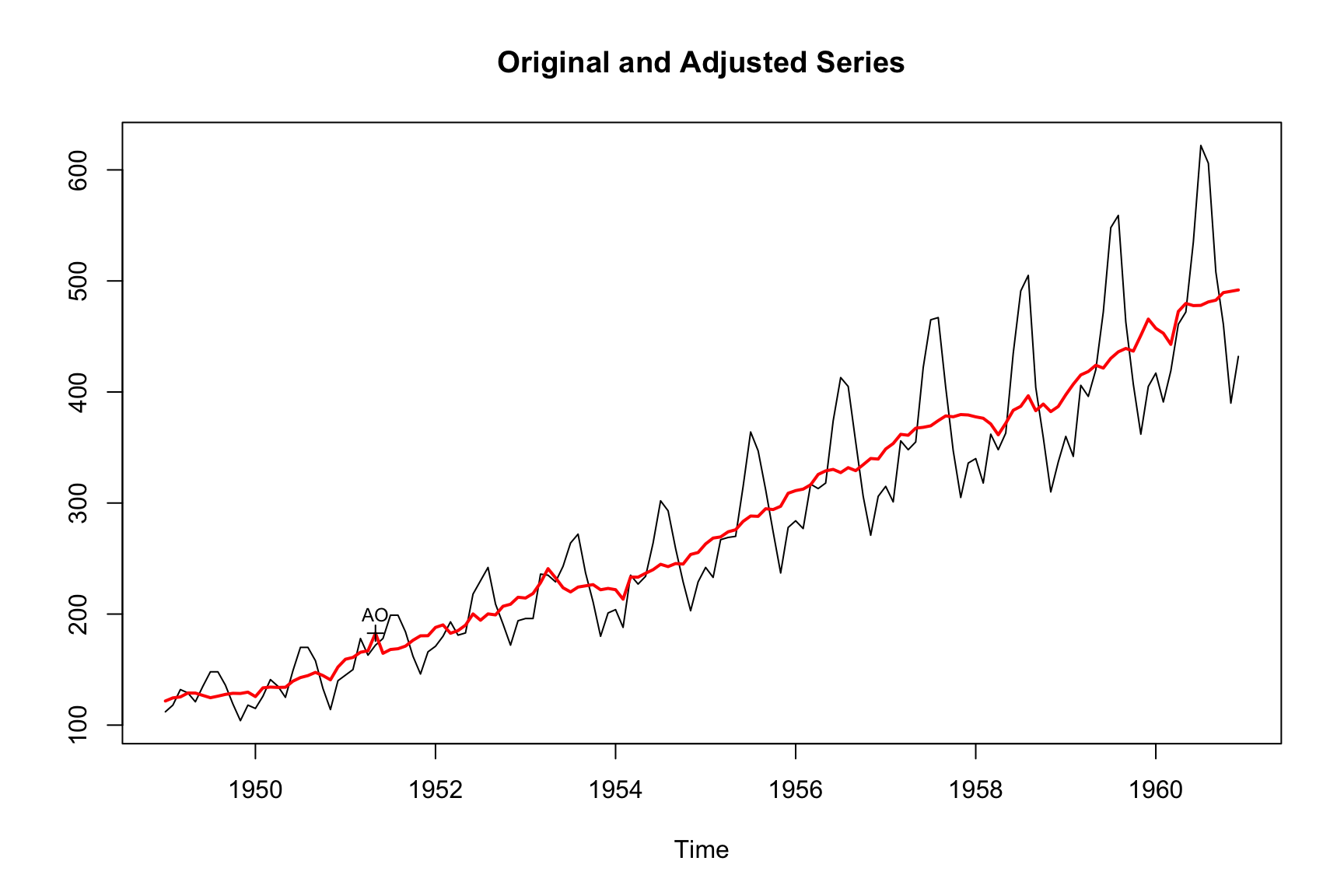
Below is our standard example. As we have seen before, the automated procedures of X-13 opt for a logarithmic transformation of the series.
m_log<-seas(AirPassengers, x11 ="")summary(m_log)#> #> Call:#> seas(x = AirPassengers, x11 = "")#> #> Coefficients:#> Estimate Std. Error z value Pr(>|z|) #> Weekday -0.0029497 0.0005232 -5.638 1.72e-08 ***#> Easter[1] 0.0177674 0.0071580 2.482 0.0131 * #> AO1951.May 0.1001558 0.0204387 4.900 9.57e-07 ***#> MA-Nonseasonal-01 0.1156204 0.0858588 1.347 0.1781 #> MA-Seasonal-12 0.4973600 0.0774677 6.420 1.36e-10 ***#> ---#> Signif. codes: 0 '***' 0.001 '**' 0.01 '*' 0.05 '.' 0.1 ' ' 1#> #> X11 adj. ARIMA: (0 1 1)(0 1 1) Obs.: 144 Transform: log#> AICc: 947.3, BIC: 963.9 QS (no seasonality in final): 0 #> Box-Ljung (no autocorr.): 26.65 Shapiro (normality): 0.9908 #> Messages generated by X-13:#> Warnings:#> - Visually significant seasonal and trading day peaks have#> been found in one or more of the estimated spectra.plot(m_log)
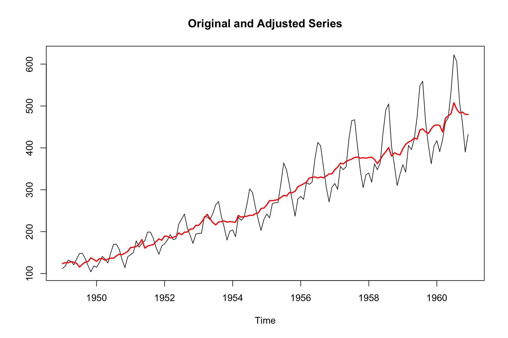
If we manually override the transformation function to be "none", this results in a very different model and seasonal adjustment. Not only are the model specification and the coefficients very different, the resulting series has a much higher volatility in later years.
m_none<-seas(AirPassengers, x11 ="", transform.function ="none")summary(m_none)#> #> Call:#> seas(x = AirPassengers, transform.function = "none", x11 = "")#> #> Coefficients:#> Estimate Std. Error z value Pr(>|z|) #> Constant 30.62077 4.60956 6.643 3.08e-11 ***#> Leap Year 11.32104 3.43088 3.300 0.000968 ***#> Weekday -0.90361 0.17787 -5.080 3.77e-07 ***#> Easter[1] 6.89372 1.80972 3.809 0.000139 ***#> AR-Nonseasonal-01 0.81929 0.04903 16.709 < 2e-16 ***#> ---#> Signif. codes: 0 '***' 0.001 '**' 0.01 '*' 0.05 '.' 0.1 ' ' 1#> #> X11 adj. ARIMA: (1 0 0)(0 1 0) Obs.: 144 Transform: none#> AICc: 993.4, BIC: 1010 QS (no seasonality in final):0.4593 #> Box-Ljung (no autocorr.): 29.2 Shapiro (normality): 0.984 #> Messages generated by X-13:#> Warnings:#> - At least one visually significant trading day peak has been#> found in one or more of the estimated spectra.plot(m_none)
Why is the transformation function so important?
In fact, applying a logarithmic transformation is equivalent to estimating a multiplicative seasonal adjustment model. This is one of the most fundamental decisions during seasonal adjustment.
4.1 Additive and multiplicative adjustment
As you remember from Chapter 1, Seasonal adjustment decomposes a time series into a trend, a seasonal, and an irregular component. Algebraically, the fundamental identity of seasonal adjustment looks like this:
\[Y_t = T_t + S_t + I_t. \tag{4.1}\]
We seek the decompose our observed series \(Y_t\) into a trend \(T_t\), a seasonal \(S_t\), and an irregular \(I_t\) component. The formulation above is additive, i.e., the trend, the seasonal, and the irregular component sum up to the observed series. The goal of seasonal adjustment is to subtract the seasonal component:
\[A_t = Y_t - S_t.\]
For example, an observed value of 100 with a seasonal compontent of -3.2 would result in a seasonally adjusted value of 100 - 3.2 = 96.8.
Alternatively, the decomposition can be multiplicative:
\[Y_t = T_t \cdot S_t \cdot I_t \tag{4.2}\]
I.e., the observed series is the product of the trend and the seasonal and irregular components. Since these are factors, the goal of seasonal adjustment is to remove seasonality by dividing by the seasonal factor.
\[A_t = \frac{Y_t}{S_t}.\]
For example, an observed value of 100 with a seasonal factor of 1.08 would result in a seasonally adjusted value of 100 / 1.08 = 92.6. In a multiplicative model, values of \(S_t > 1\) decrease the observed value, and \(S_t < 1\) increase it.
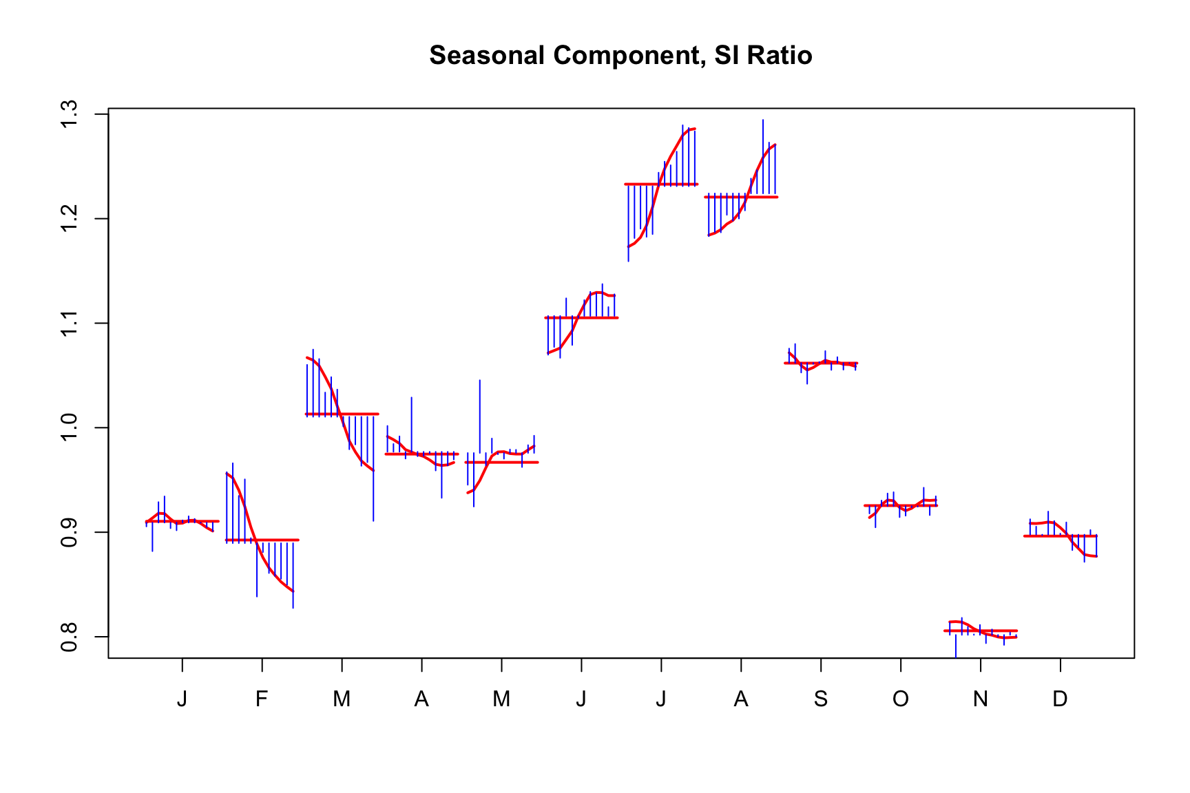
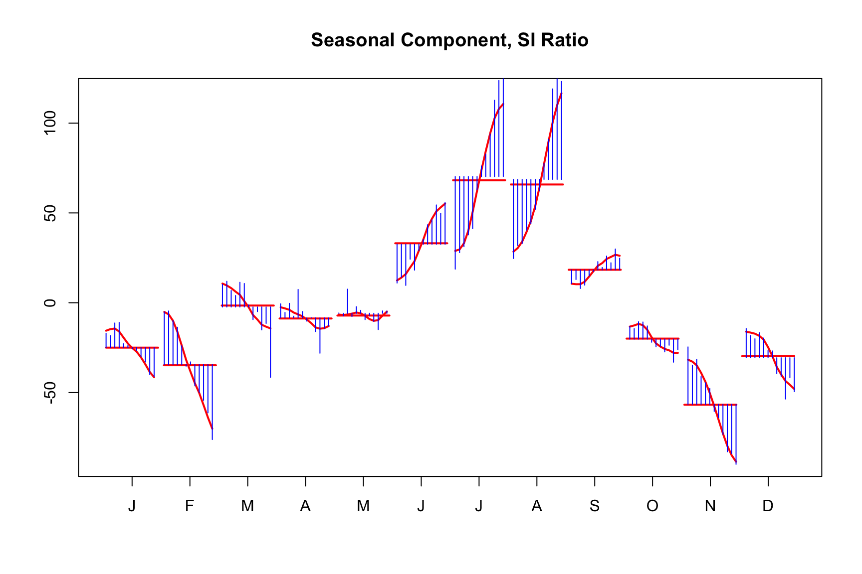
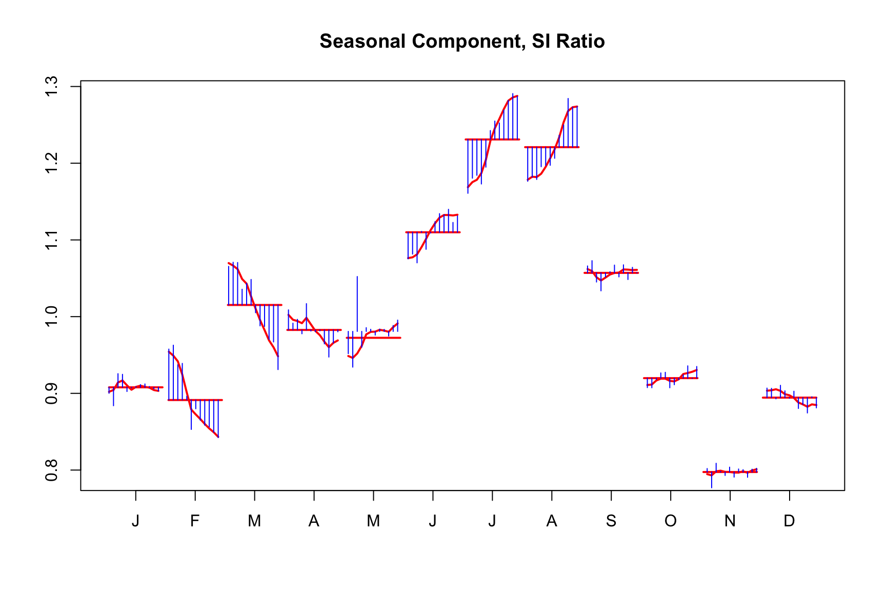
When analyzing seasonal components, the transformation is crucial. For example, monthplot() plots the evolution of the seasonal component for each period over time (shown by the evolving red line; the red bar shows its average). If the model is multiplicative, the seasonal component is a factor ranging from 0.8 to about 1.3. If the model is additive, the seasonal component is a summand ranging from about -100 airpassengers to about +130.
For a multiplicative adjustment, it is sufficient to apply logarithms to the initial series and then re-transform the results following the decomposition. With no transformation, X-13 will perform an additive seasonal adjustment as specified in Equation 4.1. With log transformation, X-13 will perform a multiplicative adjustment as specified in Equation 4.2.
4.2 Automated transformation choice
X-13 has a built-in statistical test determine the appropriateness of applying logarithmic transformation. The choice is made by comparing the AICc1 value of an ARIMA (0 1 1)(0 1 1) model (or, optionally, a user-specified model) to the log-transformed series and the original series.
1 With small sample sizes, a standard AIC test may select models with too many parameters. AICc tackles this problem by correcting for sample size.
For most practical purposes, the automatic selection mechanism is quite reliable and can be trusted to make the appropriate choice. However, if your data series contains negative values, logarithmic transformation is not feasible, and the software will automatically adapt its selection process accordingly.
To examine the outcomes of these transformation tests, one can refer to specific statistics: The udg() function grants access to broad array of diagnostic statistics. The qs() function and the AIC(), BIC() and logLik() methods are wrappers that use udg() to access some specific diagnostic statistics. For example, if we want to access the AICc values that were used to determine the appropriateness of the logarithmic model, we use:
The AICc for the log transformed model is lower than the for the untransformed one. That is why the automated procedure has selected a log transformation, as we have seen previously in Chapter 2.
4.3 Prior modifications
Prior modifications describe a second, less commonly used transformation in X-13. A prior modification scales each observation for known fixed effects. These effects can be well-known and established, such as the length of a period or leap-year effects, or they can be more subjective such as a modification for a workers’ strike.
We can think of prior-modification factors as events or corrections made to your data that are fixed throughout the adjustment process. These prior modification factors can also be permanent (default) or temporary. Permanent modifications are excluded from the final seasonal adjustment. Temporary modifications are removed while calculating seasonal factors but added back to the seasonally adjusted series.
In most cirumstances, incorporating external effects in a seasonal adjustment model would be left to the regression part in regARIMA, and will be covered in Chapter 5.
4.4 Transform options
Frequently used spec arguments in the transform spec
Arguments
Description
Example values
transform.function
Transform function
none, log, auto
transform.aicdiff
adjust tolerance of AIC test for log transform
-2, 0, 3
xtrans
Prior adjustment factor
The transform spec controls these options. Some primary options within this spec are
4.5 Case Study: AirPassengers
Why does AirPassengers seem to follow a multiplicative model of seasonal adjusmtent? The answer is heteroskadasticity, or a varying variance. As the number of air passengers grow over time, so does their seasonality. With just a few people flying, we would expect the seasonal component to be small in absolute numbers. With many people using airplanes, the seasonal component is bigger in absolute numbers. In such a series, it makes more sense describe seasonality in a multiplicative model, and thus to log tranform the series before modeling.
This is a characteric of many economic time series, wich often exibit a growth in the trend.
This is also a good place to get our first look at the seasonal factors. The monthplot() method offers a convenient way to look at these:
Like the R base monthplot() function that can be applied on any time series (also on quarterly time series!), this groups time series data by months. If you look at the January (J), entry, the blue bars show the evolution of the detrended data from 1949 to 1960. The red bar shows the average seasonal factor over these years. The smooth red lines show the seasonal factors as estimated by the model.
As you can see from the plot, there are more passengers during the summer months and fewer in the winter. The seasonal factors change over time. The summer peak becomes more pronounced in later years, while the local peak in February and March disappears over time.
If you want to extract the seasonal factor directly into R, you can use the series() function:
series(m, "seats.seasonal")
4.6 Case Study: A more difficult decision
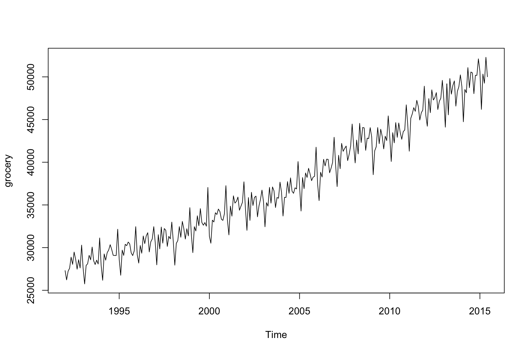
Consider the situation where you are trying to decide on transform choices for monthly retail grocery store data. The series grocery is part of the seasonalbook package.
Visual inspection of the series shows no immediate reason to think we need to perform a logarithmic transform. There is possible seasonal heteroskadasity which could be mitigated by taking logs. Perform an X-11 adjustment with all the defaults of seasonal
This is interesting since the AICc for no transformation is lower than the AICc for log transform.
transformfunction(m)#> [1] "log"
The default value for transform.aicdiff is -2, meaning the program slightly prefers log transform, and the difference between the AICc values must exceed 2. In this situation, the difference between the AICc values is -1.917597. Suppose you were to change this option to transform.aicdiff = 0, then the program selects no transform.
Perform a seasonal adjustment on the AirPassengers data using the default settings. Plot the results. Which transformation has been applied?
Then, perform the same seasonal adjustment but override the transformation function to be "none". Plot the results.
Compare the plots and describe how the transformation affects the seasonally adjusted series.
Interpreting AICc values:
Perform a seasonal adjustment on the AirPassengers data using the default settings.
Use the udg() function to access the AICc values for both the log-transformed and the untransformed models. Compare these values and explain why the log transformation was chosen by the automated procedure.
Exploring additive and multiplicative models:
Perform a seasonal adjustment on the AirPassengers data using both additive and multiplicative models by specifying the appropriate transformation functions.
Use the monthplot() function to visualize the seasonal components for both models. Compare the seasonal components and discuss how they differ between the additive and multiplicative models.
Deciding on a transformation:
Perform a seasonal adjustment on the grocery data using the default settings.
Compute the AICc values for both the log-transformed and the untransformed models using the udg() function. Compare these values and explain which transformation would be more appropriate based on the AICc values.
Experiment with changing the transform.aicdiff option to see how it affects the transformation choice.