m <- seas(AirPassengers)
summary(m)
#>
#> Call:
#> seas(x = AirPassengers)
#>
#> Coefficients:
#>                     Estimate Std. Error z value Pr(>|z|)
#> Weekday           -0.0029497  0.0005232  -5.638 1.72e-08 ***
#> Easter[1]          0.0177674  0.0071580   2.482   0.0131 *
#> AO1951.May         0.1001558  0.0204387   4.900 9.57e-07 ***
#> MA-Nonseasonal-01  0.1156204  0.0858588   1.347   0.1781
#> MA-Seasonal-12     0.4973600  0.0774677   6.420 1.36e-10 ***
#> ---
#> Signif. codes:  0 '***' 0.001 '**' 0.01 '*' 0.05 '.' 0.1 ' ' 1
#>
#> SEATS adj.  ARIMA: (0 1 1)(0 1 1)  Obs.: 144  Transform: log
#> AICc: 947.3, BIC: 963.9  QS (no seasonality in final):    0
#> Box-Ljung (no autocorr.): 26.65 Shapiro (normality): 0.99088 Irregular holidays
Many time series are affected by public holidays. For example, retail sales typically increase before Christmas, and are much lower during Christmas days. Similar effects occur for Chinese New Year, Ramadan, Diwali or Easter. In seasonal adjustment, the treatment of Christmas is usually not much of a problem because Christmas always occurs on the same date in December. Thus, the Christmas effect is simply part of the December effect (or of the fourth quarter effect, if you have a quarterly series).
Things are more complicated with irregular holidays. Because their occurrence follows different rules, the holiday happens at different months in different years. Easter, for example, is based on the lunar cycles of the Jewish calendar, and is sometimes in March and sometimes in April. In quarterly data, Easter falls either in the first or in the second quarter.
For the interpretation of many time series, this constitutes a problem. Retails sales, for example, are usually reduced during the Easter holiday. If March values are compared between years, their interpretation depends on the exact day of Easter. If Easter falls into March, we would expect lower retail sales in this month. Conversely, if it falls into April, we would expect April numbers to be lower.
regression.variables that are relevant for holiday adjustment
| Variable | Description |
|---|---|
easter[w] |
Easter holiday regression variable for monthly or quarterly flow data that assumes the level of daily activity changes on the w-th day before Easter and remains at the new level through the day before Easter. This value w must be supplied and can range from 1 to 25. A user can also specify an easter[0] regression variable, which assumes the daily level of activity level changes only on Easter Sunday. To estimate complex effects, several of these variables, differing in their choices of w, can be specified. |
labor[w] |
Labor Day holiday regression variable (monthly flow data only) that assumes the level of daily activity changes on the w-th day before Labor Day and remains at the new level until the day before Labor Day. The value w must be supplied and can range from 1 to 25. |
thank[w] |
Thanksgiving holiday regression variable (monthly flow data only) that assumes the level of daily activity changes on the w-th day before or after Thanksgiving and remains at the new level until December 24. The value w must be supplied and can range from −8 to 17. Values of w < 0 indicate a number of days after Thanksgiving; values of w > 0 indicate a number of days before Thanksgiving. |
8.1 Automated Adjustment
By default, seas() calls the automated routines to detect Easter effects in a series. For example, the default call detects an Easter effect with a length of one in the air passengers time series:
X-13 tests various lengths of an Easter effect and picks the one model with the lowest AICc. Easter[1] indicates that a length of one day has been chosen. I.e., the Easter holiday period is thought to start on Easter day and last for only one day. Alternatively, Easter[8] starts at Easter day and lasts for the eight subsequent days. If we want to enforce an eight-day Easter holiday, we can specify the call as follows:
m_easter_8 <- seas(AirPassengers, regression.variables = "easter[8]")
summary(m_easter_8)
#>
#> Call:
#> seas(x = AirPassengers, regression.variables = "easter[8]")
#>
#> Coefficients:
#>                     Estimate Std. Error z value Pr(>|z|)
#> Weekday           -0.0028967  0.0005289  -5.477 4.33e-08 ***
#> Easter[8]          0.0158629  0.0074253   2.136   0.0327 *
#> AO1951.May         0.1008171  0.0206437   4.884 1.04e-06 ***
#> MA-Nonseasonal-01  0.1215690  0.0858086   1.417   0.1566
#> MA-Seasonal-12     0.5036477  0.0770917   6.533 6.44e-11 ***
#> ---
#> Signif. codes:  0 '***' 0.001 '**' 0.01 '*' 0.05 '.' 0.1 ' ' 1
#>
#> SEATS adj.  ARIMA: (0 1 1)(0 1 1)  Obs.: 144  Transform: log
#> AICc: 948.8, BIC: 965.4  QS (no seasonality in final):    0
#> Box-Ljung (no autocorr.):  26.4   Shapiro (normality): 0.9895
Surprisingly, the 8-day Easter model has a lower AICc than the one-day model. This opens the question of why the one-day model has been chosen in the beginning.
Including holiday effects can have a dramatic effect on a final seasonal adjustment. Consider the monthly retail sales from Hobby, toy, and game stores. The data can be found at the US Census Time Series repository.
How to read data from CENSUS into R
get_census_time_series <- function(url) {
tf <- tempfile(fileext = ".txt")
download.file(census_url, tf)
ans <- readr::read_csv(tf, skip = 6, col_types = cols(
Period = col_character(),
Value = col_double()
))
ans |>
mutate(
month.abb = gsub("\\-.+$", "", Period),
year = gsub("^.+\\-", "", Period)
) |>
left_join(tibble(month.abb, month = seq(month.abb)), by = join_by(month.abb)) |>
mutate(time = as.Date(paste(year, month, 1, sep = "-"))) |>
select(time, value = Value) |>
filter(!is.na(value)) |>
tsbox::ts_ts()
}
census_url <- "https://www.census.gov/econ_export/?format=csv&adjusted=true¬Adjusted=false&errorData=false&mode=report&default=&errormode=Dep&charttype=&chartmode=&chartadjn=&submit=GET+DATA&program=MARTS&startYear=1992&endYear=2023&categories%5B0%5D=44X72&dataType=SM&geoLevel=US"
get_census_time_series(census_url)ts_plot(hobby_toy_game, title = "Hobby, Toy and Game store monthly sales")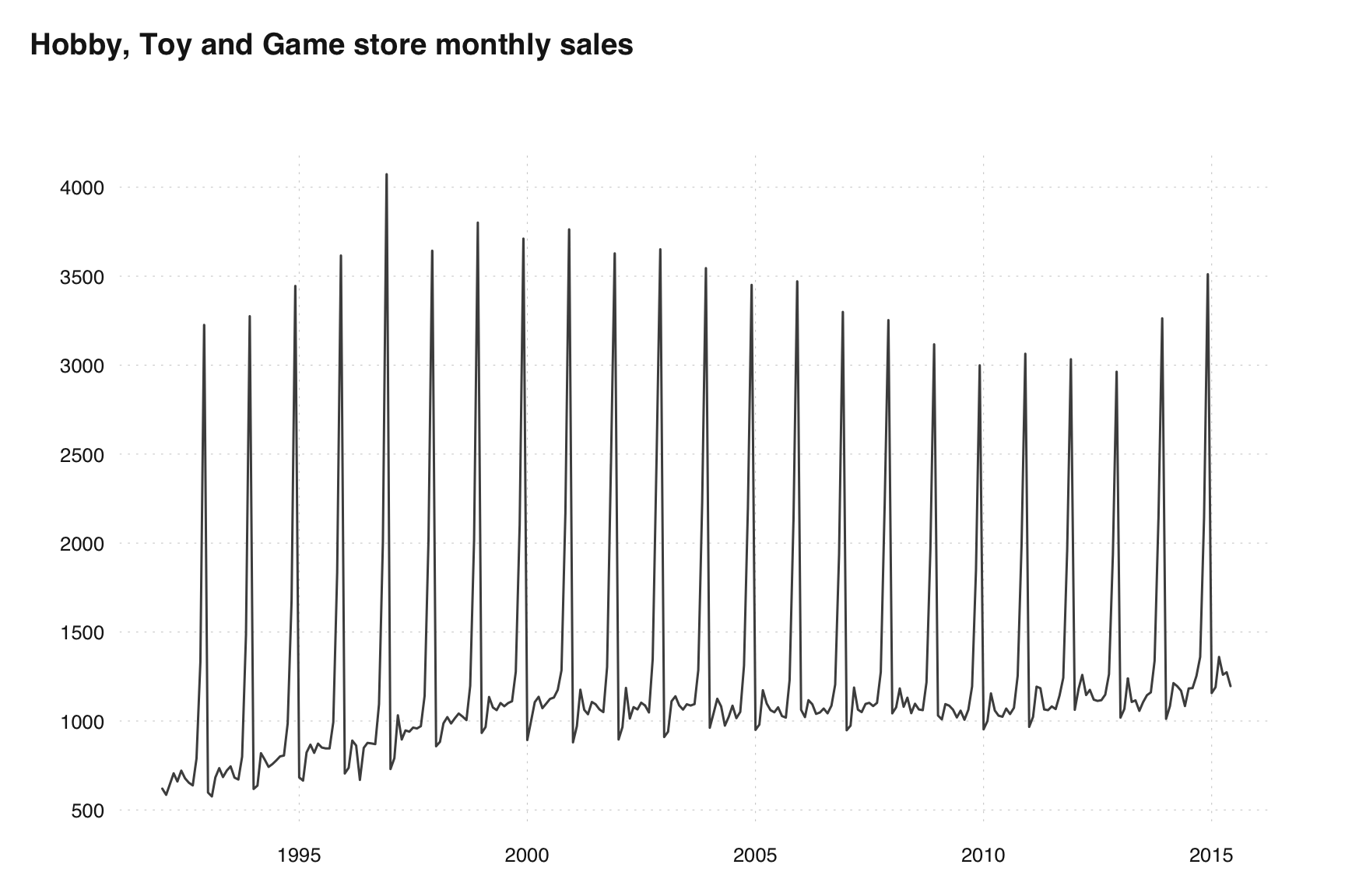
We can perform a seasonal adjustment on this series with and without the Easter[8] regressor.
m0 <- seas(hobby_toy_game, x11 = "", regression = NULL, outlier = NULL)
m1 <- seas(hobby_toy_game, x11 = "", regression.variables = "Easter[8]", outlier = NULL)
ts_dygraphs(
  ts_c(
    hobby_toy_game, SA_noEaster = final(m0), SA_withEaster = final(m1)
  )
)
Notice the large differences during certain Easter periods. For example, the final seasonally adjusted series including an Easter regressor in April 2011 was 1360.52. The final seasonally adjusted values without an Easter regressor was 1449.3, a difference of 89 million dollars which more than 7.5% higher than the original series value. Moreover, including the Easter regressor resulted in a smoother seasonally adjusted series.
8.2 Case Study: Chinese New Year
The Lunar New Year is the most important holiday in China and many other Asian countries. Traditionally, the holiday starts on Lunar New Year’s Eve, and lasts until the Lantern Festival on the 15th day of the first month of the lunisolar calendar. The Chinese New Year is celebrated either in January or in February of the Gregorian calendar.
Because of its importance, Chinese New Year seriously distorts monthly time series, which are usually reported according to the Gregorian calendar. Unlike Easter, Chinese New Year does not affect quarterly time series, as it always falls in the first quarter.
X-13-ARIMA-SEATS has a built-in adjustment procedure for the Easter holiday, but not for Chinese New Year. However, all packages allow for the inclusion of user-defined variables, and the Chinese New Year can be modeled as such.
8.2.1 Imports of Goods to China
Chinese imports are included as an example series in seasonalbook, both with and without the official seasonal adjustment.
library(tsbox)
stopifnot(packageVersion("seasonalbook") >= "0.0.2")
ts_plot(imp_cn)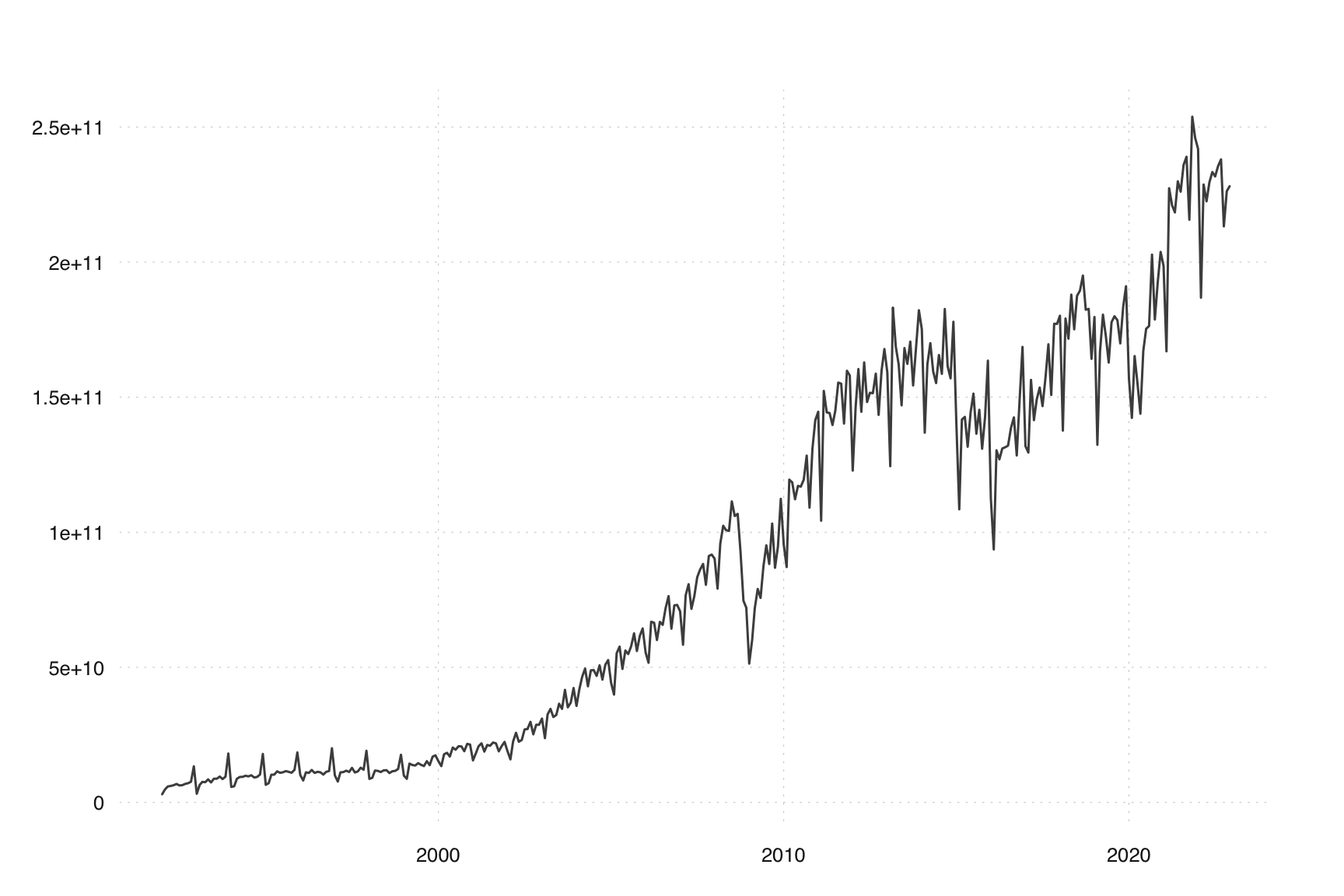
The series has a very different seasonal pattern before 2000, we focus on the later period. (Adjusting the whole series in one step is possible, but for good results one should manually model the seasonal break.)
imp_cn_2000 <- ts_span(imp_cn, start = 2000)ts_dygraphs() works similar to ts_plot(), but allows for zooming:
ts_dygraphs(imp_cn_2000)
How to read data from FRED into R
fredr provides access to the Federal Reserve of Economic Data (FRED), provided by the Federal Reserve Bank of St. Louis. To use fredr and the FRED API in general, you must first obtain a FRED API key. Take a look at the Documentation for details.
The core function in this package is fredr(), which fetches observations for a FRED series.
We can use purrr::map_dfr() to download multiple series at once:
A bit of tidying:
imp_cn_tidy <-
  imp_cn_raw |>
  select(time = date, id = series_id, value) |>
  mutate(id = recode(
    id,
    XTIMVA01CNM667S = "sa",
    XTIMVA01CNM667N = "nsa"
  ))
Use the tsbox package to convert the data frame into ts objects.
Both time series are included in the book package.
library(seasonalbook)
imp_cn_sa
imp_cn
seasonal includes the genhol() function, a R version of the equally named software utility by the U.S. Census Bureau. Using the dates of the Chinese New Year as an input, it produces a time series with the deviations from the monthly means. Here we are assuming that the holiday starts on New Year’s Eve and lasts for one week.
reg_cny <- genhol(cny, start = -1, end = 6, center = "calendar")
tsbox::ts_dygraphs(reg_cny)
The center argument normalizes the series by either subtracting the overall average effect ("mean") or the average for each period ("calendar"). You should use "calendar" for Easter or Chinese New Year, but "mean" for Ramadan. Without this adjustment ("none"), the holiday effect is subtracted, altering the annual value of the series.
8.2.2 Including user-defined regressors
The time series reg_cny can be included in the main seasonal adjustment. The automated procedures of X-13ARIMA-SEATS can be applied to the imp series in the following way:
m1 <- seas(
  imp_cn,
  xreg = reg_cny,
  regression.usertype = "holiday",
  x11 = list()
)
summary(m1)
#>
#> Call:
#> seas(x = imp_cn, xreg = reg_cny, regression.usertype = "holiday",
#>     x11 = list())
#>
#> Coefficients:
#>                     Estimate Std. Error z value Pr(>|z|)
#> xreg              -0.1763689  0.0126544 -13.937  < 2e-16 ***
#> Weekday            0.0074166  0.0009114   8.138 4.02e-16 ***
#> AO1999.Dec        -0.2066833  0.0505465  -4.089 4.33e-05 ***
#> LS2008.Nov        -0.3898401  0.0528219  -7.380 1.58e-13 ***
#> MA-Nonseasonal-01  0.4537545  0.0469504   9.665  < 2e-16 ***
#> MA-Seasonal-12     0.3143759  0.0485684   6.473 9.62e-11 ***
#> ---
#> Signif. codes:  0 '***' 0.001 '**' 0.01 '*' 0.05 '.' 0.1 ' ' 1
#>
#> X11 adj.  ARIMA: (0 1 1)(0 1 1)  Obs.: 372  Transform: log
#> AICc: 1.693e+04, BIC: 1.695e+04  QS (no seasonality in final):    0
#> Box-Ljung (no autocorr.): 26.03   Shapiro (normality): 0.9704 ***
plot(m1)
With xreg, arbitrary user-defined regressors can be included, regression.usertype = "holiday" ensures that the final series does not include the regression effect. We also have chosen X11 as the decomposition method.
Unsurprisingly, the summary reveals a highly significant Chinese New Year effect. As the automatic model has been estimated on the logarithmic series, the coefficient of -0.17 indicates that New Year in 2023 will lower imports in January, by approximately 0.74 * 17 ~ 13% (compared to average January), and increase it by the same amount in February. The automatic procedure has also detected weekday effects and a level shift during the financial crisis.
8.2.3 Multiple regressors
We can do even better by using more than one user-defined regressors, one for the pre-New-Year period and one for the post-New-Year period:
pre_cny <- genhol(cny, start = -6, end = -1, frequency = 12, center = "calendar")
post_cny <- genhol(cny, start = 0, end = 6, frequency = 12, center = "calendar")
m2 <- seas(
  imp_cn,
  xreg = ts_c(pre_cny, post_cny),
  regression.usertype = "holiday",
  x11 = list()
)
summary(m2)
#>
#> Call:
#> seas(x = imp_cn, xreg = ts_c(pre_cny, post_cny), regression.usertype = "holiday",
#>     x11 = list())
#>
#> Coefficients:
#>                    Estimate Std. Error z value Pr(>|z|)
#> xreg1              0.008910   0.015179   0.587    0.557
#> xreg2             -0.186830   0.018563 -10.065  < 2e-16 ***
#> Weekday            0.007404   0.000906   8.172 3.04e-16 ***
#> AO1999.Dec        -0.206691   0.050272  -4.111 3.93e-05 ***
#> LS2008.Nov        -0.388900   0.052698  -7.380 1.58e-13 ***
#> MA-Nonseasonal-01  0.450334   0.046985   9.585  < 2e-16 ***
#> MA-Seasonal-12     0.313567   0.048553   6.458 1.06e-10 ***
#> ---
#> Signif. codes:  0 '***' 0.001 '**' 0.01 '*' 0.05 '.' 0.1 ' ' 1
#>
#> X11 adj.  ARIMA: (0 1 1)(0 1 1)  Obs.: 372  Transform: log
#> AICc: 1.693e+04, BIC: 1.696e+04  QS (no seasonality in final):    0
#> Box-Ljung (no autocorr.): 27.37   Shapiro (normality): 0.9687 ***
plot(m2)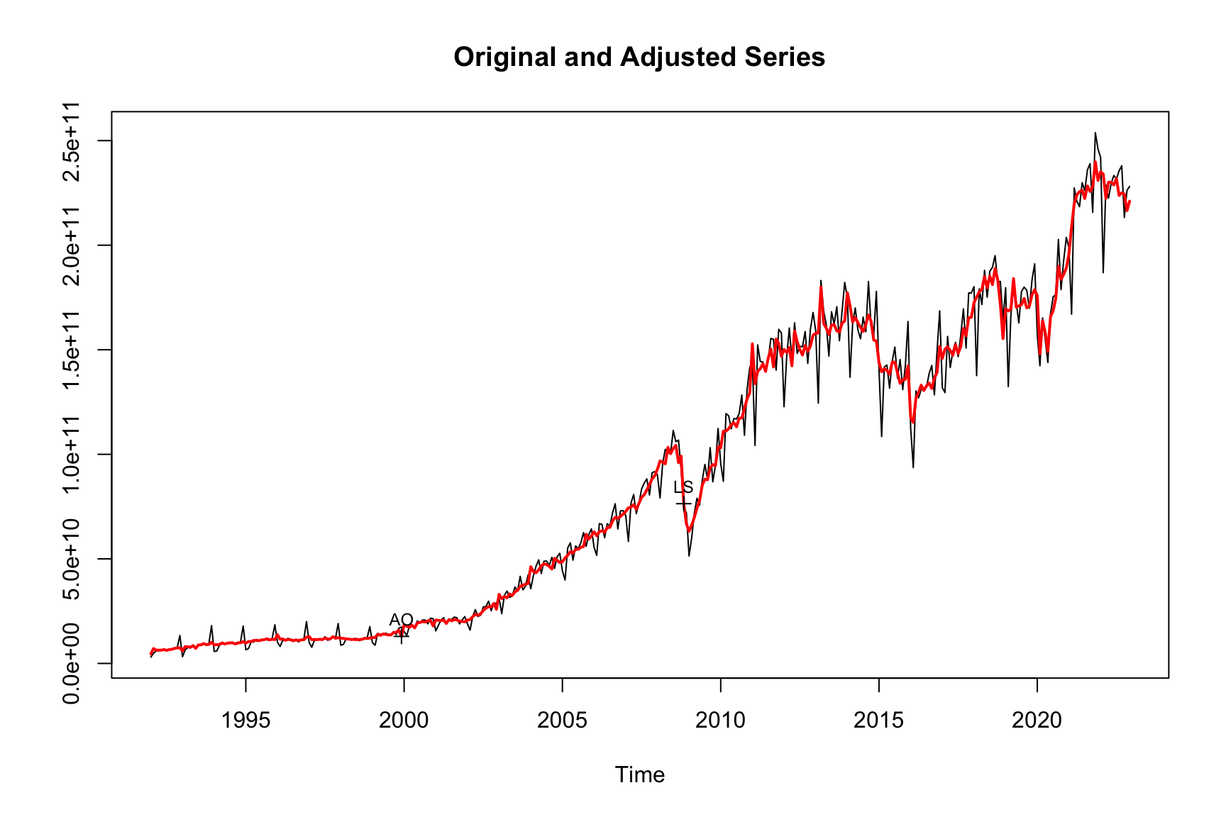
8.2.4 Compare with official adjustments
I haven’t done any research on how the officially seasonally adjusted rates are computed, but they seem very close to a default call to seas(). Our models (both m1, but especially m2), does a much better job of adjusting to Chinese New Year.
ts_dygraphs(
  ts_c(
    cny = ts_span(reg_cny * 1e11 + 1e11, start = 2000, end = 2024),
    ts_pick(imp_cn_2000, "sa"),
    final(seas(x = imp_cn, x11 = "")),
    final(m2)
  )
)
Replicate automated Easter adjustment in R
We can use R’s arima() function and genhol() to fully replicate X-13’s automated Easter adjustment.
Let’s build an Easter regressor, using genhol():
And use this in an ARIMA model in R:
arima(
  log(AirPassengers),
  order = c(0,1,1),
  seasonal = c(0,1,1),
  xreg = ea
)
#>
#> Call:
#> arima(x = log(AirPassengers), order = c(0, 1, 1), seasonal = c(0, 1, 1), xreg = ea)
#>
#> Coefficients:
#>           ma1     sma1      ea
#>       -0.3772  -0.5493  0.0200
#> s.e.   0.0930   0.0735  0.0099
#>
#> sigma^2 estimated as 0.00131:  log likelihood = 246.65,  aic = -485.29
Now, let’s compare to the results of X-13:
m <- seas(
  AirPassengers,
  regression.variables = c("easter[1]"),
  regression.aictest = NULL
)
summary(m)
#>
#> Call:
#> seas(x = AirPassengers, regression.aictest = NULL, regression.variables = c("easter[1]"))
#>
#> Coefficients:
#>                   Estimate Std. Error z value Pr(>|z|)
#> Easter[1]         0.019990   0.009936   2.012   0.0442 *
#> MA-Nonseasonal-01 0.377151   0.079753   4.729 2.26e-06 ***
#> MA-Seasonal-12    0.549333   0.076650   7.167 7.68e-13 ***
#> ---
#> Signif. codes:  0 '***' 0.001 '**' 0.01 '*' 0.05 '.' 0.1 ' ' 1
#>
#> SEATS adj.  ARIMA: (0 1 1)(0 1 1)  Obs.: 144  Transform: log
#> AICc: 985.6, BIC: 996.8  QS (no seasonality in final):    0
#> Box-Ljung (no autocorr.): 29.93   Shapiro (normality): 0.9931
#> Messages generated by X-13:
#> Warnings:
#> - At least one visually significant trading day peak has been
#>   found in one or more of the estimated spectra.
Note that R defines the ARIMA model with negative signs before the MA term, X-13 with a positive sign.
8.3 Case Study: Azerbaijani Retail Sales
library(cbar.sa)
#>
#> Attaching package: 'cbar.sa'
#> The following object is masked _by_ '.GlobalEnv':
#>
#> m1
#> The following object is masked from 'package:seasonal':
#>
#> cpi
library(seasonal)
library(dplyr)
# manual regressor construction
ramadan_ts_manual <-
islamic_calendar |>
group_by(y = lubridate::year(date)) |>
mutate(ramadan_y = sum(ramadan)) |>
ungroup() |>
group_by(y = lubridate::year(date), q = lubridate::quarter(date)) |>
summarize(time = date[1], value = sum(ramadan) / ramadan_y[1], .groups = "drop") |>
select(time, value) |>
tsbox::ts_ts()
# Careful, this is not centered!
# ### automatic regressor construction (experimental)
ramadan <-
islamic_calendar |>
mutate(diff = ramadan - lag(ramadan)) |>
mutate(start = (diff == 1)) |>
dplyr::filter(start) |>
pull(date)
# Q: Can we come up with a defined start date for Ramadan or Muharrem?
islamic_calendar |>
filter(date %in% c("2000-11-26", "2000-11-27", "2000-11-28"))
#> [90m# A tibble: 3 × 3[39m
#> [1mdate[22m [1mmuharrem[22m [1mramadan[22m
#> [3m[90m<date>[39m[23m [3m[90m<dbl>[39m[23m [3m[90m<dbl>[39m[23m
#> [90m1[39m 2000-11-26 0 0
#> [90m2[39m 2000-11-27 0 1
#> [90m3[39m 2000-11-28 0 1
# Q: Is the length of Ramadan uniquely defined?
ramadan_ts_auto <- seasonal::genhol(ramadan, frequency = 4, start = 0, end = 29, center = "none")
# Applying the calendar mean adjustment
ramadan_ts <- seasonal::genhol(ramadan, frequency = 4, start = 0, end = 29, center = "mean")
# Different pattern pre 2008
plot(trade_tur)
m0 <- seas(trade_tur, x11 = "")
m1 <- seas(
trade_tur,
xreg = ramadan_ts,
regression.usertype = "holiday"
)
summary(m0)
#>
#> Call:
#> seas(x = trade_tur, x11 = "")
#>
#> Coefficients:
#> Estimate Std. Error z value Pr(>|z|)
#> LS2008.2 0.08703 0.01820 4.783 1.73e-06 ***
#> LS2009.1 -0.09009 0.01820 -4.951 7.38e-07 ***
#> AO2015.2 0.06888 0.01132 6.087 1.15e-09 ***
#> AR-Nonseasonal-01 0.29250 0.10936 2.675 0.00748 **
#> ---
#> Signif. codes: 0 '***' 0.001 '**' 0.01 '*' 0.05 '.' 0.1 ' ' 1
#>
#> X11 adj. ARIMA: (1 1 0)(0 1 0) Obs.: 82 Transform: log
#> AICc: 971.7, BIC: 982.6 QS (no seasonality in final):0.5095
#> Box-Ljung (no autocorr.): 27.15 Shapiro (normality): 0.9653 *
summary(m1) # xreg insignificant
#>
#> Call:
#> seas(x = trade_tur, xreg = ramadan_ts, regression.usertype = "holiday")
#>
#> Coefficients:
#> Estimate Std. Error z value Pr(>|z|)
#> xreg 0.01230 0.01058 1.162 0.24526
#> LS2008.2 0.08789 0.01804 4.871 1.11e-06 ***
#> LS2009.1 -0.09371 0.01834 -5.111 3.20e-07 ***
#> AO2015.2 0.06956 0.01119 6.215 5.14e-10 ***
#> AR-Nonseasonal-01 0.29861 0.10884 2.744 0.00608 **
#> ---
#> Signif. codes: 0 '***' 0.001 '**' 0.01 '*' 0.05 '.' 0.1 ' ' 1
#>
#> SEATS adj. ARIMA: (1 1 0)(0 1 0) Obs.: 82 Transform: log
#> AICc: 972.7, BIC: 985.6 QS (no seasonality in final): 0
#> Box-Ljung (no autocorr.): 26.64 Shapiro (normality): 0.9566 *
# If we start adjusting from 2008 on, we get a better result
m2 <- seas(trade_tur, x11 = "", series.modelspan = "2008.01,")
m3 <- seas(
trade_tur,
xreg = ramadan_ts,
regression.usertype = "holiday",
series.modelspan = "2008.01,"
)
summary(m2)
#>
#> Call:
#> seas(x = trade_tur, x11 = "", series.modelspan = "2008.01,")
#>
#> Coefficients:
#> Estimate Std. Error z value Pr(>|z|)
#> AO2008.1 -0.127442 0.021218 -6.006 1.90e-09 ***
#> AO2015.2 0.069109 0.008652 7.988 1.37e-15 ***
#> LS2020.2 -0.055809 0.014080 -3.964 7.38e-05 ***
#> AR-Nonseasonal-01 0.368127 0.124057 2.967 0.003 **
#> ---
#> Signif. codes: 0 '***' 0.001 '**' 0.01 '*' 0.05 '.' 0.1 ' ' 1
#>
#> X11 adj. ARIMA: (1 1 0)(0 1 0) Obs.: 82 Transform: log
#> AICc: 739.7, BIC: 748.7 QS (no seasonality in final): 0
#> Box-Ljung (no autocorr.): 25.72 Shapiro (normality): 0.9259 **
summary(m3)
#>
#> Call:
#> seas(x = trade_tur, xreg = ramadan_ts, regression.usertype = "holiday",
#> series.modelspan = "2008.01,")
#>
#> Coefficients:
#> Estimate Std. Error z value Pr(>|z|)
#> xreg 0.028760 0.008556 3.362 0.000775 ***
#> AO2008.1 -0.126803 0.018087 -7.011 2.37e-12 ***
#> LS2012.1 -0.045014 0.011856 -3.797 0.000147 ***
#> AO2015.2 0.069747 0.007173 9.724 < 2e-16 ***
#> LS2020.2 -0.054681 0.011856 -4.612 3.99e-06 ***
#> MA-Nonseasonal-01 -0.404526 0.121835 -3.320 0.000899 ***
#> ---
#> Signif. codes: 0 '***' 0.001 '**' 0.01 '*' 0.05 '.' 0.1 ' ' 1
#>
#> SEATS adj. ARIMA: (0 1 1)(0 1 0) Obs.: 82 Transform: log
#> AICc: 726.6, BIC: 738.6 QS (no seasonality in final):0.03671
#> Box-Ljung (no autocorr.): 28.13 Shapiro (normality): 0.9629 .
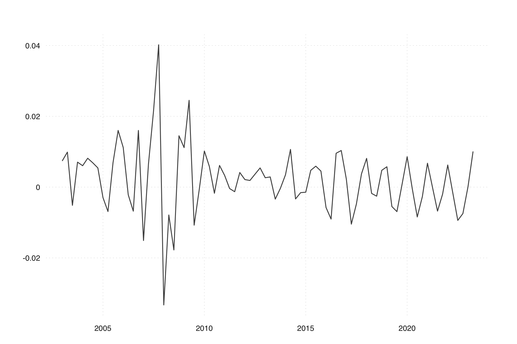
tsbox::ts_plot(
delta_perc = (final(m3) - final(m2)) / final(m2)
)
# Applying the calendar mean adjustment
ramadan_pre_ts <- seasonal::genhol(ramadan, frequency = 4, start = -2, end = 0, center = "mean")
library(tsbox)
m4 <- seas(
trade_tur,
xreg = cbind(ramadan_pre_ts, ramadan_ts),
regression.usertype = "holiday",
series.modelspan = "2008.01,"
)
# Q: Does the sign makes sense?
summary(m4)
#>
#> Call:
#> seas(x = trade_tur, xreg = cbind(ramadan_pre_ts, ramadan_ts),
#> regression.usertype = "holiday", series.modelspan = "2008.01,")
#>
#> Coefficients:
#> Estimate Std. Error z value Pr(>|z|)
#> xreg1 -0.010146 0.004235 -2.396 0.0166 *
#> xreg2 0.036534 0.008445 4.326 1.52e-05 ***
#> AO2008.1 -0.131754 0.017178 -7.670 1.72e-14 ***
#> LS2012.1 -0.042722 0.010156 -4.206 2.59e-05 ***
#> AO2015.2 0.071251 0.006030 11.817 < 2e-16 ***
#> LS2020.2 -0.054455 0.010156 -5.362 8.23e-08 ***
#> MA-Nonseasonal-01 -0.483042 0.116524 -4.145 3.39e-05 ***
#> MA-Seasonal-04 -0.144730 0.132190 -1.095 0.2736
#> ---
#> Signif. codes: 0 '***' 0.001 '**' 0.01 '*' 0.05 '.' 0.1 ' ' 1
#>
#> SEATS adj. ARIMA: (0 1 1)(0 1 1) Obs.: 82 Transform: log
#> AICc: 726.5, BIC: 741 QS (no seasonality in final):0.1123
#> Box-Ljung (no autocorr.): 22.75 Shapiro (normality): 0.9542 *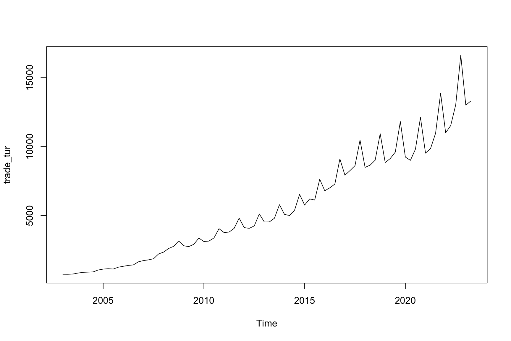
8.4 Exercises
Go through
seasonal::genhol()documentation and make sure you understand its argument.Can you replicate
seasonal::genhol(easter, frequency = 4, start = -2, center = "calendar")output manually?Can you explain why do we need to set
center = "mean"for Ramadan?What is the consequence of not specifying
regression.usertype = "holiday"in a call toseas()when adjusting for moving holidays?