library(tsbox)
stopifnot(packageVersion("seasonalbook") >= "0.0.2")
library(seasonalbook)
library(seasonal)

ts_plot(imp_cn)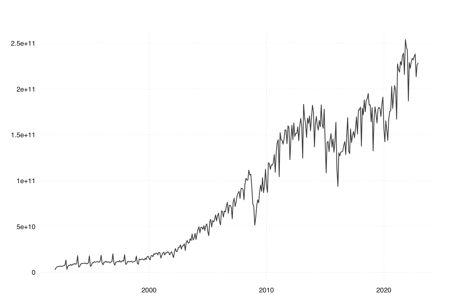
The goal of seasonal adjustment is to remove repeating seasonal patterns from time series data. These patterns are predictable and can be modeled in an ARIMA model. A seasonal break refers to a sudden change in the seasonal pattern of the data. Such a change could be due to various factors, such as:
A major economic event that alters consumer behavior or business operations, leading to long-lasting change in the seasonal component.
A change in policy or regulations that affects the seasonal cycle, such as new holiday schedules or school calendars.
Shifts in consumer preferences that change the way people interact with products or services throughout the year.
Changes in how the data is measured or surveyed, e.g, changes in the population being surveyed, or revisions to the methodologies used to gather the data.
Detecting seasonal breaks is important because they can significantly affect the accuracy of the underlying ARIMA model.
In the case of the SEATS method, the ARIMA model will affect both the ARIMA forecast and the seasonal adjustment.
In case of the X-11 method, the moving averages are capable of dealing with changes in the seasonal pattern. The shorter the filter, the faster they adapt to an altered sesaonal pattern. However, the X-11 method is also susceptible to seasonal breaks, since ARIMA forecast is needed at the margin of the series.
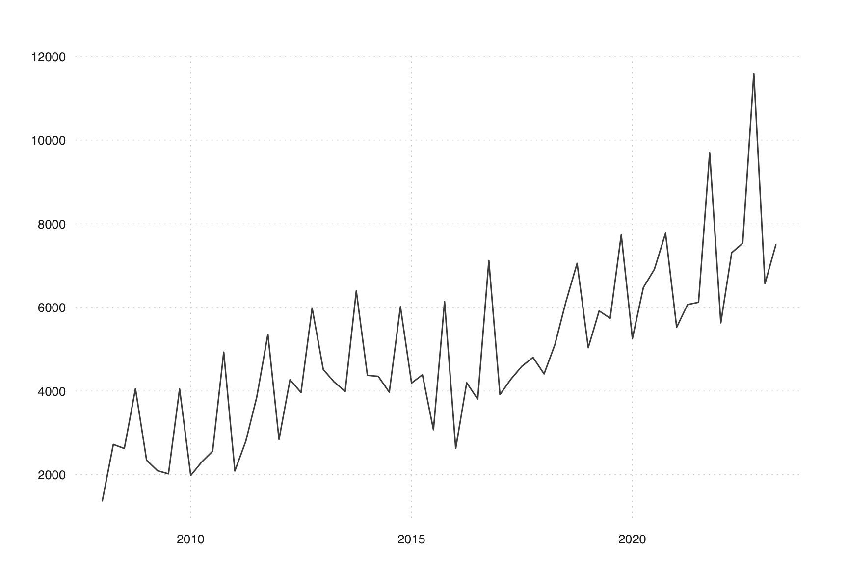
In a previous case study, we analyzed the imports of goods to China, where we detected a pretty obvious seasonal break.
Chinese imports are included as an example series in seasonal, both with and without the official seasonal adjustment.
library(tsbox)
stopifnot(packageVersion("seasonalbook") >= "0.0.2")
library(seasonalbook)
library(seasonal)
ts_plot(imp_cn)
As can be spotted quickly, the series has a very different seasonal pattern before 2000. In our previous example, we simply cut the data and focused on the later period.
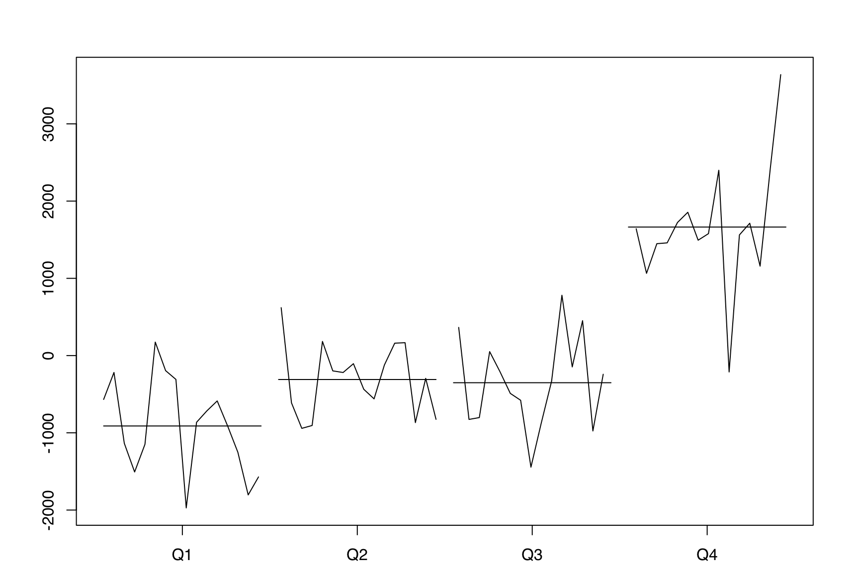
The seasonal break is even clearer to spot in the monthplot of the series:
This makes it obvious that there were very strong December effects before 2000. We don’t know anything about the series, but we can speculate that prior to 2000, custom receipts were counted at the end of the year, rather than at the date of import.
We can put in a change of regime regression variable that allows for different seasonal regressors before and after January 2000. This regression variable is discussed in more detail below in Section 11.3.
m = seas(
  imp_cn,
  x11 = "",
  regression.variables = c("seasonal/2000.1/"),
  regression.aictest = NULL,
  outlier = NULL,
  transform.function = "log"
)
summary(m)
#>
#> Call:
#> seas(x = imp_cn, transform.function = "log", regression.aictest = NULL,
#>     outlier = NULL, x11 = "", regression.variables = c("seasonal/2000.1/"))
#>
#> Coefficients:
#>                     Estimate Std. Error z value Pr(>|z|)
#> Jan               -0.0654535  0.0181009  -3.616 0.000299 ***
#> Feb               -0.1970206  0.0180950 -10.888  < 2e-16 ***
#> Mar                0.0356460  0.0181169   1.968 0.049119 *
#> Apr                0.0328228  0.0181109   1.812 0.069937 .
#> May               -0.0238587  0.0180941  -1.319 0.187307
#> Jun                0.0067156  0.0180789   0.371 0.710295
#> Jul                0.0354693  0.0180731   1.963 0.049699 *
#> Aug                0.0350369  0.0180802   1.938 0.052641 .
#> Sep                0.0813043  0.0180989   4.492 7.05e-06 ***
#> Oct               -0.0441661  0.0181234  -2.437 0.014811 *
#> Nov                0.0328833  0.0181436   1.812 0.069926 .
#> Jan I             -0.3183942  0.0352764  -9.026  < 2e-16 ***
#> Feb I             -0.1122450  0.0350760  -3.200 0.001374 **
#> Mar I             -0.0295122  0.0350251  -0.843 0.399452
#> Apr I             -0.0286242  0.0348917  -0.820 0.412005
#> May I              0.0669706  0.0347657   1.926 0.054062 .
#> Jun I              0.0165824  0.0347032   0.478 0.632768
#> Jul I             -0.0001398  0.0347261  -0.004 0.996788
#> Aug I             -0.0354610  0.0348208  -1.018 0.308495
#> Sep I             -0.0641267  0.0349392  -1.835 0.066449 .
#> Oct I              0.0496035  0.0349988   1.417 0.156398
#> Nov I              0.0332059  0.0348833   0.952 0.341142
#> Constant           0.0098924  0.0030076   3.289 0.001005 **
#> MA-Nonseasonal-01  0.6490499  0.0510055  12.725  < 2e-16 ***
#> MA-Nonseasonal-02 -0.1976993  0.0507758  -3.894 9.88e-05 ***
#> MA-Seasonal-12    -0.2451488  0.0506633  -4.839 1.31e-06 ***
#> ---
#> Signif. codes:  0 '***' 0.001 '**' 0.01 '*' 0.05 '.' 0.1 ' ' 1
#>
#> X11 adj.  ARIMA: (0 1 2)(0 0 1)  Obs.: 372  Transform: log
#> AICc: 1.76e+04, BIC: 1.77e+04  QS (no seasonality in final):    0
#> Box-Ljung (no autocorr.): 25.25   Shapiro (normality): 0.9328 ***
#> Messages generated by X-13:
#> Warnings:
#> - At least one visually significant trading day peak has been
#>   found in one or more of the estimated spectra.
#>
#> Notes:
#> - Stable seasonal regressors present in the regARIMA model.
#>   Maximum seasonal difference in automatic model
#>   identification procedure set to zero.
The coefficients from the summary are as follows:
| Month | Pre 2000 coefficients | Post 2000 coefficients |
|---|---|---|
| Jan | -0.0654535 | -0.3183942 |
| Feb | -0.1970206 | -0.1122450 |
| Mar | 0.0356460 | -0.0295122 |
| Apr | 0.0328228 | -0.0286242 |
| May | -0.0238587 | 0.0669706 |
| Jun | 0.0067156 | 0.0165824 |
| Jul | 0.0354693 | -0.0001398 |
| Aug | 0.0350369 | -0.0354610 |
| Sep | 0.0813043 | -0.0641267 |
| Oct | -0.0441661 | 0.0496035 |
| Nov | 0.0328833 | 0.0332059 |
| Dec (derived) | -0.0294782 | 0.3710507 |
We see multiple sign changes and multiple large discrepancies between the two model spans. This is an indication that this series has a change-of-regime. Also as previously indicated the December effect was much different post 2000.
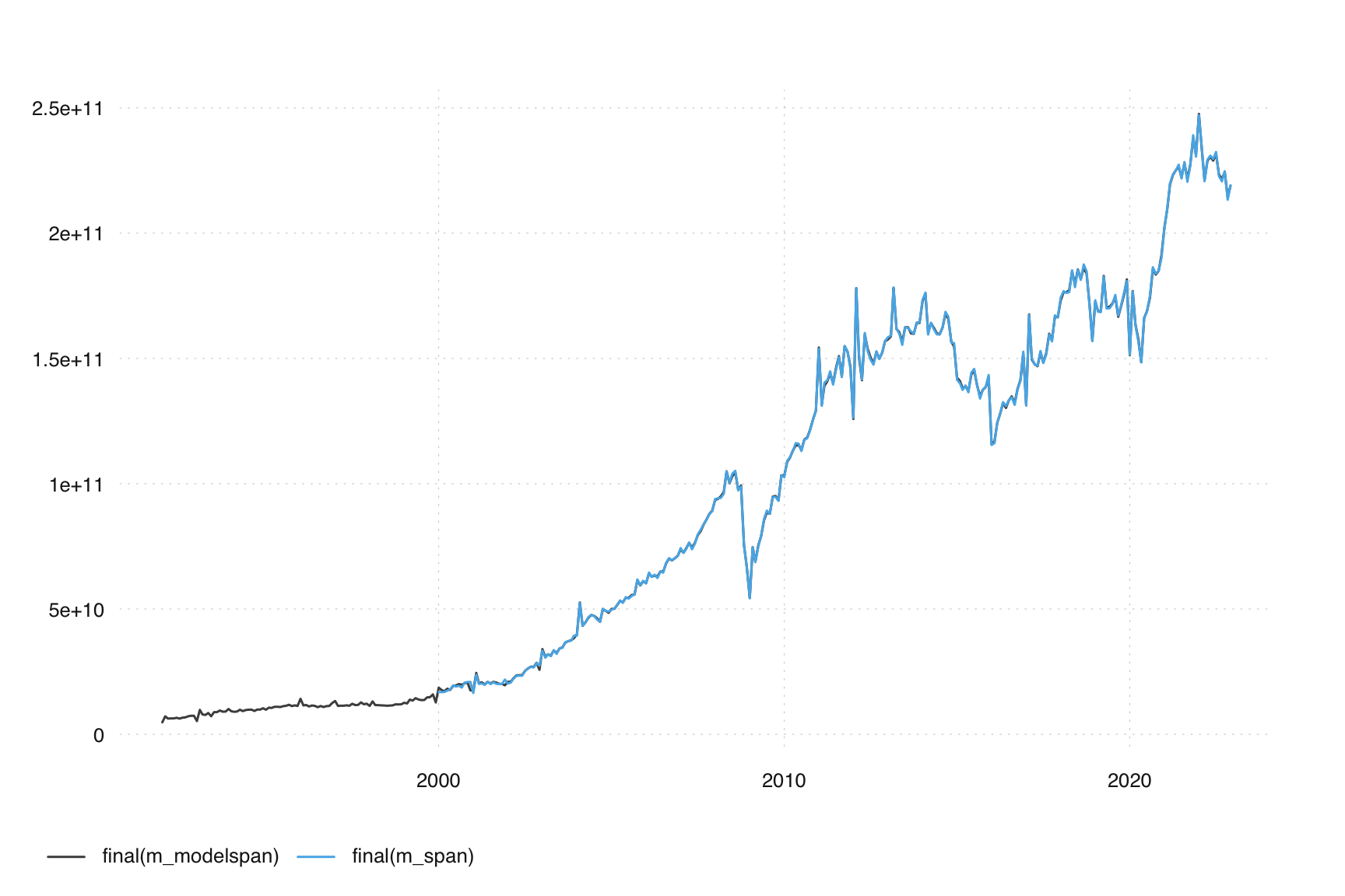
In many cases, restricting series.modelspan may be the easiest way to deal with such series.
When restricting the model span, we use only part of the series for model estimation, but still applies seasonal adjustment to the whole series. Thus, the ARIMA model is the same as if we cutted the span of the series before adjustment (as we did in the previous case study):
m_modelspan <- seas(
  imp_cn,
  series.modelspan = "2000.jan,",
  x11 = list()
)
summary(m_modelspan)
#>
#> Call:
#> seas(x = imp_cn, series.modelspan = "2000.jan,", x11 = list())
#>
#> Coefficients:
#>                    Estimate Std. Error z value Pr(>|z|)
#> AO2001.Jan        -0.261726   0.043878  -5.965 2.45e-09 ***
#> AO2004.Feb         0.218728   0.042608   5.133 2.84e-07 ***
#> LS2008.Nov        -0.327482   0.047759  -6.857 7.03e-12 ***
#> AO2009.Jan        -0.280528   0.042369  -6.621 3.56e-11 ***
#> AO2011.Jan         0.153783   0.042806   3.593 0.000328 ***
#> AO2012.Jan        -0.169644   0.043482  -3.901 9.56e-05 ***
#> AO2012.Feb         0.174648   0.043120   4.050 5.11e-05 ***
#> LS2016.Jan        -0.229816   0.047847  -4.803 1.56e-06 ***
#> Weekday            0.006700   0.000806   8.313  < 2e-16 ***
#> AR-Nonseasonal-01 -0.426105   0.054515  -7.816 5.44e-15 ***
#> MA-Seasonal-12     0.794516   0.040311  19.710  < 2e-16 ***
#> ---
#> Signif. codes:  0 '***' 0.001 '**' 0.01 '*' 0.05 '.' 0.1 ' ' 1
#>
#> X11 adj.  ARIMA: (1 1 0)(0 1 1)  Obs.: 372  Transform: log
#> AICc: 1.258e+04, BIC: 1.262e+04  QS (no seasonality in final):    0
#> Box-Ljung (no autocorr.): 31.39   Shapiro (normality): 0.9949

m_span <- seas(
  ts_span(imp_cn, "2000-01"),
  x11 = list()
)
summary(m_span)
#>
#> Call:
#> seas(x = ts_span(imp_cn, "2000-01"), x11 = list())
#>
#> Coefficients:
#>                    Estimate Std. Error z value Pr(>|z|)
#> AO2001.Jan        -0.261726   0.043878  -5.965 2.45e-09 ***
#> AO2004.Feb         0.218728   0.042608   5.133 2.84e-07 ***
#> LS2008.Nov        -0.327482   0.047759  -6.857 7.03e-12 ***
#> AO2009.Jan        -0.280528   0.042369  -6.621 3.56e-11 ***
#> AO2011.Jan         0.153783   0.042806   3.593 0.000328 ***
#> AO2012.Jan        -0.169644   0.043482  -3.901 9.56e-05 ***
#> AO2012.Feb         0.174648   0.043120   4.050 5.11e-05 ***
#> LS2016.Jan        -0.229816   0.047847  -4.803 1.56e-06 ***
#> Weekday            0.006700   0.000806   8.313  < 2e-16 ***
#> AR-Nonseasonal-01 -0.426105   0.054515  -7.816 5.44e-15 ***
#> MA-Seasonal-12     0.794516   0.040311  19.710  < 2e-16 ***
#> ---
#> Signif. codes:  0 '***' 0.001 '**' 0.01 '*' 0.05 '.' 0.1 ' ' 1
#>
#> X11 adj.  ARIMA: (1 1 0)(0 1 1)  Obs.: 276  Transform: log
#> AICc: 1.258e+04, BIC: 1.262e+04  QS (no seasonality in final):    0
#> Box-Ljung (no autocorr.): 31.39   Shapiro (normality): 0.9949
By using the series.modelspan, we restrict the data used in the ARIMA model, but we sill adjust the whole series. This leads to almost the same seasonally adjusted series in the overlapping period (after 2000).
Note that the ARIMA model that has been chosen is not optimal for the period before 2000. This will affect the backcast of the series, and may lead to slighly sub-optimal results for the first year. Since the interest in the accuracy of the latest data is usually much higher, this seems like a good compromise in many cases.
A way to ‘model’ seasonal breaks to include seasonal dummies before (and possibly after) the supposed break. A seasonal dummy model can be estimated by an appropriate specification of the regression.variables argument. This is done with a so-called change-of-regime regression variable. There are two types of change-of-regime regressors available: full and partial.
Change of regime regressors are denoted by adding the change date, enclosed in one or two slashes. This designated date divides the series under analysis into two periods: an early span encompassing data prior to the change date, and a late span covering data from this date onwards.
| Type | Syntax | Example |
|---|---|---|
| Full change of regime regressor | reg/date/ |
seasonal/2000.jan/ |
| Partial change of regime regressor, zero before change date | reg//date/ |
seasonal//2000.jan/ |
| Partial change of regime regressor, zero on and after change date | reg/date// |
sesaonal/2000.jan// |
To model the span after 2000, we can either cut the time series input (as we did in the case study), or use the series.span argument:
m1 <- seas(
  imp_cn,
  outlier = NULL,
  x11 = "",
  arima.model = "(0 1 1)",
  transform.function = "log",
  regression.variables = "seasonal",
  series.span = "2000.jan,"
)
summary(m1)
#>
#> Call:
#> seas(x = imp_cn, transform.function = "log", outlier = NULL,
#>     x11 = "", arima.model = "(0 1 1)", regression.variables = "seasonal",
#>     series.span = "2000.jan,")
#>
#> Coefficients:
#>                    Estimate Std. Error z value Pr(>|z|)
#> Jan               -0.068265   0.013106  -5.209 1.90e-07 ***
#> Feb               -0.203522   0.013082 -15.558  < 2e-16 ***
#> Mar                0.033622   0.013063   2.574  0.01006 *
#> Apr                0.033961   0.013048   2.603  0.00925 **
#> May               -0.023603   0.013039  -1.810  0.07027 .
#> Jun                0.008008   0.013033   0.614  0.53896
#> Jul                0.039197   0.013035   3.007  0.00264 **
#> Aug                0.035561   0.013041   2.727  0.00640 **
#> Sep                0.086085   0.013049   6.597 4.19e-11 ***
#> Oct               -0.042614   0.013063  -3.262  0.00111 **
#> Nov                0.033393   0.013083   2.552  0.01070 *
#> Weekday            0.006096   0.001137   5.362 8.24e-08 ***
#> MA-Nonseasonal-01  0.342034   0.056700   6.032 1.62e-09 ***
#> ---
#> Signif. codes:  0 '***' 0.001 '**' 0.01 '*' 0.05 '.' 0.1 ' ' 1
#>
#> X11 adj.  ARIMA: (0 1 1)  Obs.: 276  Transform: log
#> AICc: 1.326e+04, BIC: 1.33e+04  QS (no seasonality in final):    0
#> Box-Ljung (no autocorr.): 27.61   Shapiro (normality): 0.9556 ***
In order to model the span before 2000, the specification looks as follows:
m2 <- seas(
  imp_cn,
  outlier = NULL,
  x11 = "",
  arima.model = "(0 1 1)",
  transform.function = "log",
  regression.variables = "seasonal",
  series.span = ",1999.dec"
)
summary(m2)
#>
#> Call:
#> seas(x = imp_cn, transform.function = "log", outlier = NULL,
#>     x11 = "", arima.model = "(0 1 1)", regression.variables = "seasonal",
#>     series.span = ",1999.dec")
#>
#> Coefficients:
#>                    Estimate Std. Error z value Pr(>|z|)
#> Jan               -0.387506   0.033779 -11.472   <2e-16 ***
#> Feb               -0.304623   0.033613  -9.063   <2e-16 ***
#> Mar               -0.001298   0.033535  -0.039   0.9691
#> Apr               -0.007866   0.033531  -0.235   0.8145
#> May                0.048099   0.033810   1.423   0.1548
#> Jun                0.009728   0.033459   0.291   0.7712
#> Jul                0.029471   0.033391   0.883   0.3774
#> Aug                0.007545   0.033592   0.225   0.8223
#> Sep                0.005823   0.033691   0.173   0.8628
#> Oct                0.019756   0.033711   0.586   0.5578
#> Nov                0.077857   0.033614   2.316   0.0205 *
#> Weekday            0.008259   0.003786   2.182   0.0291 *
#> MA-Nonseasonal-01  0.670552   0.072772   9.214   <2e-16 ***
#> ---
#> Signif. codes:  0 '***' 0.001 '**' 0.01 '*' 0.05 '.' 0.1 ' ' 1
#>
#> X11 adj.  ARIMA: (0 1 1)  Obs.: 96  Transform: log
#> AICc:  4264, BIC:  4295  QS (no seasonality in final):6.021 *
#> Box-Ljung (no autocorr.): 45.85 ** Shapiro (normality): 0.9202 ***
Note that we set outlier, arima.model and transform.function such that we can ensure comparability.
We can use the regression.variables argument to estimate the whole span in one call:
m3 <- seas(
  imp_cn,
  outlier = NULL,
  x11 = "",
  arima.model = "(0 1 1)",
  transform.function = "log",
  regression.variables = "seasonal/2000.jan//",
)
summary(m3)
#>
#> Call:
#> seas(x = imp_cn, transform.function = "log", outlier = NULL,
#>     x11 = "", arima.model = "(0 1 1)", regression.variables = "seasonal/2000.jan//")
#>
#> Coefficients:
#>                    Estimate Std. Error z value Pr(>|z|)
#> Jan I             -0.386705   0.034705 -11.143  < 2e-16 ***
#> Feb I             -0.301462   0.034517  -8.734  < 2e-16 ***
#> Mar I              0.004075   0.034367   0.119 0.905618
#> Apr I             -0.001388   0.034268  -0.040 0.967700
#> May I              0.050501   0.034285   1.473 0.140765
#> Jun I              0.015335   0.034187   0.449 0.653745
#> Jul I              0.033103   0.034199   0.968 0.333078
#> Aug I              0.006655   0.034294   0.194 0.846126
#> Sep I              0.006256   0.034369   0.182 0.855558
#> Oct I              0.012976   0.034397   0.377 0.706007
#> Nov I              0.068627   0.034354   1.998 0.045755 *
#> Weekday            0.006342   0.001790   3.543 0.000395 ***
#> MA-Nonseasonal-01  0.559147   0.042527  13.148  < 2e-16 ***
#> ---
#> Signif. codes:  0 '***' 0.001 '**' 0.01 '*' 0.05 '.' 0.1 ' ' 1
#>
#> X11 adj.  ARIMA: (0 1 1)  Obs.: 372  Transform: log
#> AICc: 1.779e+04, BIC: 1.785e+04  QS (no seasonality in final):    0
#> Box-Ljung (no autocorr.): 248.8 *** Shapiro (normality): 0.9482 ***
By default, seasonal outliers are removed from the final series.
We can conduct an F-test for seasonality similar to those discussed in Section 12.6. Here instead of a single F-test over the whole model span, instead we look at 3 different F-tests; before the change of regime, after the change of regime and a combined test. We can find the F-test results by using the grep function over the names(udg(m)) character vector.
ftest_udg_names = grep(pattern = "ftest", names(udg(m)), value = TRUE)
ftest = udg(m, ftest_udg_names) |> t() |> round(4)
colnames(ftest) = c("df1", "df2", "test_stat", "p_val")
ftest
#>                                             df1 df2 test_stat p_val
#> ftest$Seasonal (after 2000.Jan)              11 348   16.9989     0
#> ftest$Seasonal (change for before 2000.Jan)  11 348   22.1542     0
#> ftest$Combined Seasonal Regressors 22 348 32.9303 0When should we model a seasonal break? When we have enough data after the break (as in the imports of goods to China example), restricting series.modelspan is the easiest way and leads to good results.
In some situations you may not be able to restrict the model span. For example if the seasonal break too close to the end of the series or if there is a policy restricting it. In this case, modelling the seasonal break using seasonal regressors may be an option. We apply this technique in the following Case study.
library(cbar.sa)
#>
#> Attaching package: 'cbar.sa'
#> The following object is masked _by_ '.GlobalEnv':
#>
#> m1
#> The following object is masked from 'package:seasonal':
#>
#> cpi
library(seasonal)
library(dplyr)
library(tsbox)
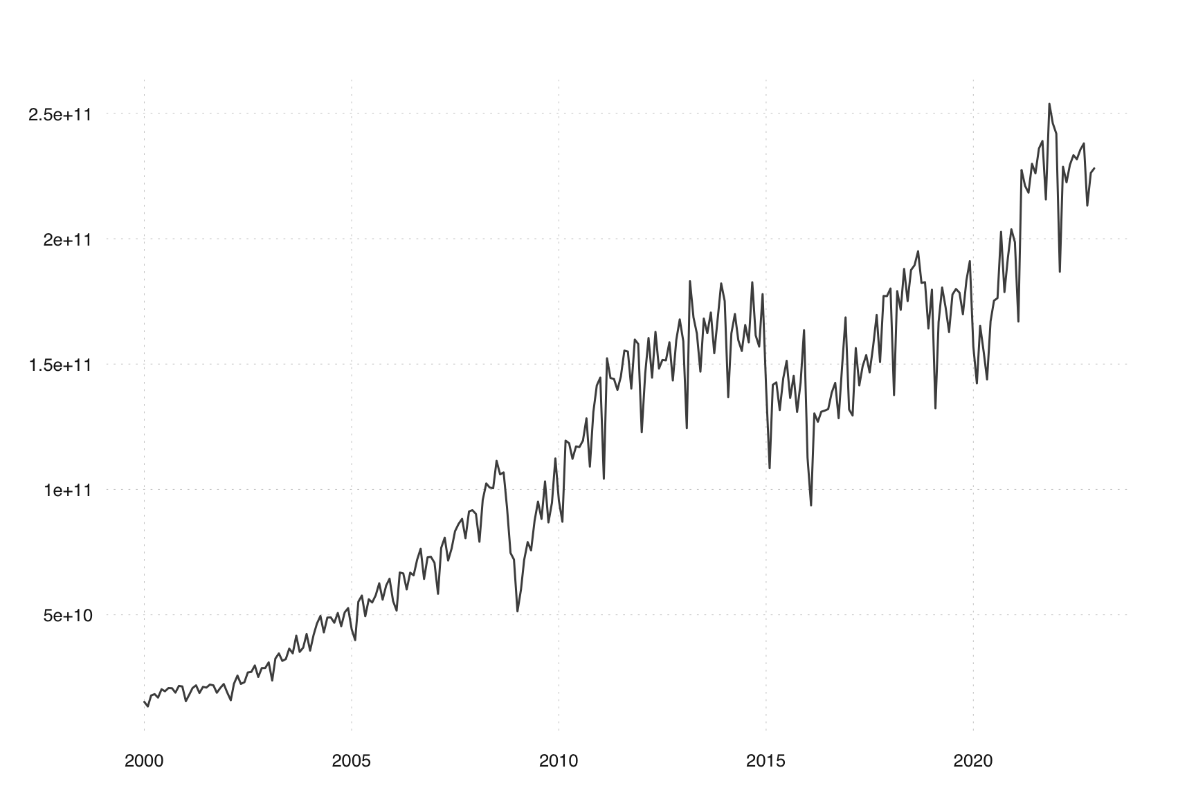
# visually not obious seasonal break
ts_plot(budg_exp)
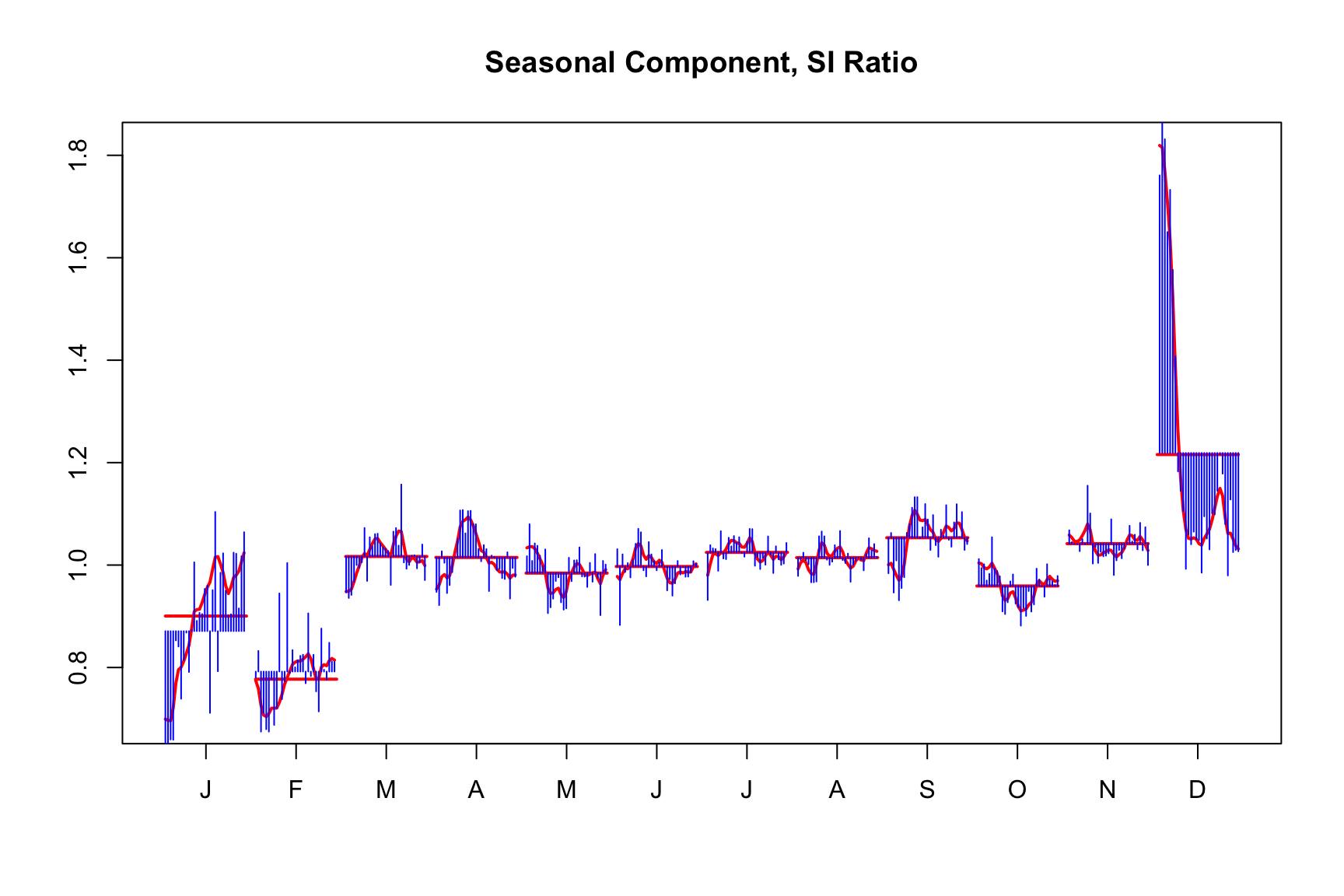
# month plot of detrended series
monthplot(budg_exp - ts_trend(budg_exp))
m1 <- seas(
x = budg_exp,
x11 = "",
regression.variables = c("const", "ao2017.4", "seasonal/2016.1/"),
arima.model = "(2 0 0)(1 0 1)",
regression.aictest = NULL,
outlier = NULL,
transform.function = "log"
)
summary(m1)
#>
#> Call:
#> seas(x = budg_exp, transform.function = "log", regression.aictest = NULL,
#> outlier = NULL, x11 = "", regression.variables = c("const",
#> "ao2017.4", "seasonal/2016.1/"), arima.model = "(2 0 0)(1 0 1)")
#>
#> Coefficients:
#> Estimate Std. Error z value Pr(>|z|)
#> Constant 8.338851 0.390244 21.368 < 2e-16 ***
#> AO2017.4 -0.336074 0.132358 -2.539 0.011113 *
#> 1st -0.217537 0.038891 -5.594 2.22e-08 ***
#> 2nd -0.042023 0.039121 -1.074 0.282732
#> 3rd -0.035355 0.040778 -0.867 0.385942
#> 1st I -0.002449 0.054689 -0.045 0.964286
#> 2nd I -0.016296 0.054168 -0.301 0.763535
#> 3rd I -0.075518 0.055309 -1.365 0.172135
#> AR-Nonseasonal-01 0.545723 0.111017 4.916 8.85e-07 ***
#> AR-Nonseasonal-02 0.417009 0.113237 3.683 0.000231 ***
#> AR-Seasonal-04 -0.152188 0.354758 -0.429 0.667930
#> MA-Seasonal-04 -0.278102 0.373339 -0.745 0.456329
#> ---
#> Signif. codes: 0 '***' 0.001 '**' 0.01 '*' 0.05 '.' 0.1 ' ' 1
#>
#> X11 adj. ARIMA: (2 0 0)(1 0 1) Obs.: 62 Transform: log
#> AICc: 1022, BIC: 1042 QS (no seasonality in final): 0
#> Box-Ljung (no autocorr.): 30.17 Shapiro (normality): 0.9883
m2 <- seas(
x = budg_exp,
x11 = "",
series.modelspan = "2016.1,",
regression.variables = c("const", "ao2017.4"),
arima.model = "(2 0 0)(1 1 1)",
regression.aictest = NULL,
outlier = NULL,
transform.function = "log"
)
m3 <- seas(
x = budg_exp,
x11 = "",
regression.variables = c("const", "ao2017.4", "seasonal/2016.1//"),
arima.model = "(2 0 0)(1 1 1)",
regression.aictest = NULL,
outlier = NULL,
transform.function = "log"
)