In the previous chapter, we got to know X-11, a seasonal decomposition procedure that utilizes predefined moving-average filters. SEATS, which we will get to know in this chapter, derives its filters from the underlying ARIMA model.
7.1 Basics
Signal Extraction in ARIMA Time Series, or SEATS, is a method for estimating unobserved components in a time series. It is developed from the work of Cleveland and Tiao (1976), Hillmer and Tiao (1982), Maravall (1986). If applied properly, SEATS seasonal factors are usually more stable than X-11, and the seasonally adjusted series show less revisions than X11 (see Section 7.7 for a more extensive discussion).
Cleveland, William P, and George C Tiao. 1976. “Decomposition of Seasonal Time Series: A Model for the Census x-11 Program.”Journal of the American Statistical Association 71 (355): 581–87.
Hillmer, S. C., and G. C. Tiao. 1982. “An ARIMA-Model-Based Approach to Seasonal Adjustment.”Journal of the American Statistical Association 77 (377): 63–70. http://www.jstor.org/stable/2287770.
Maravall, Agustin. 1986. “Revisions in ARIMA Signal Extraction.”Journal of the American Statistical Association 81 (395): 736–40. http://www.jstor.org/stable/2289005.
Like X-11, SEATS applies a series of filters to an observed time series, as described in Chapter 6. Like X-11, SEATS uses a forecast extended series, in order to obtain unbiased results at the margin. Unlike X-11, however, SEATS filters are derived from the ARIMA model of the time series. While X-11 filters are predefined and fixed, the SEATS filters are different for each ARIMA model.
While X-11 offers a finite set of filters, SEATS offers an infinite set of filters. Overall, they cover a broader set of possible filter lengths, which makes SEATS a more flexible option than X-11. The available set filter lengths is the most crucial difference between X-11 and SEATS. At the same time, the additional flexibility may lead at times to filters that are undesirable. As will be shown later on, SEATS sometimes choose a filter that is too narrow, and produces an overly volatile seasonal component.
To perform a SEATS seasonal adjustment in R, you can use the following code:
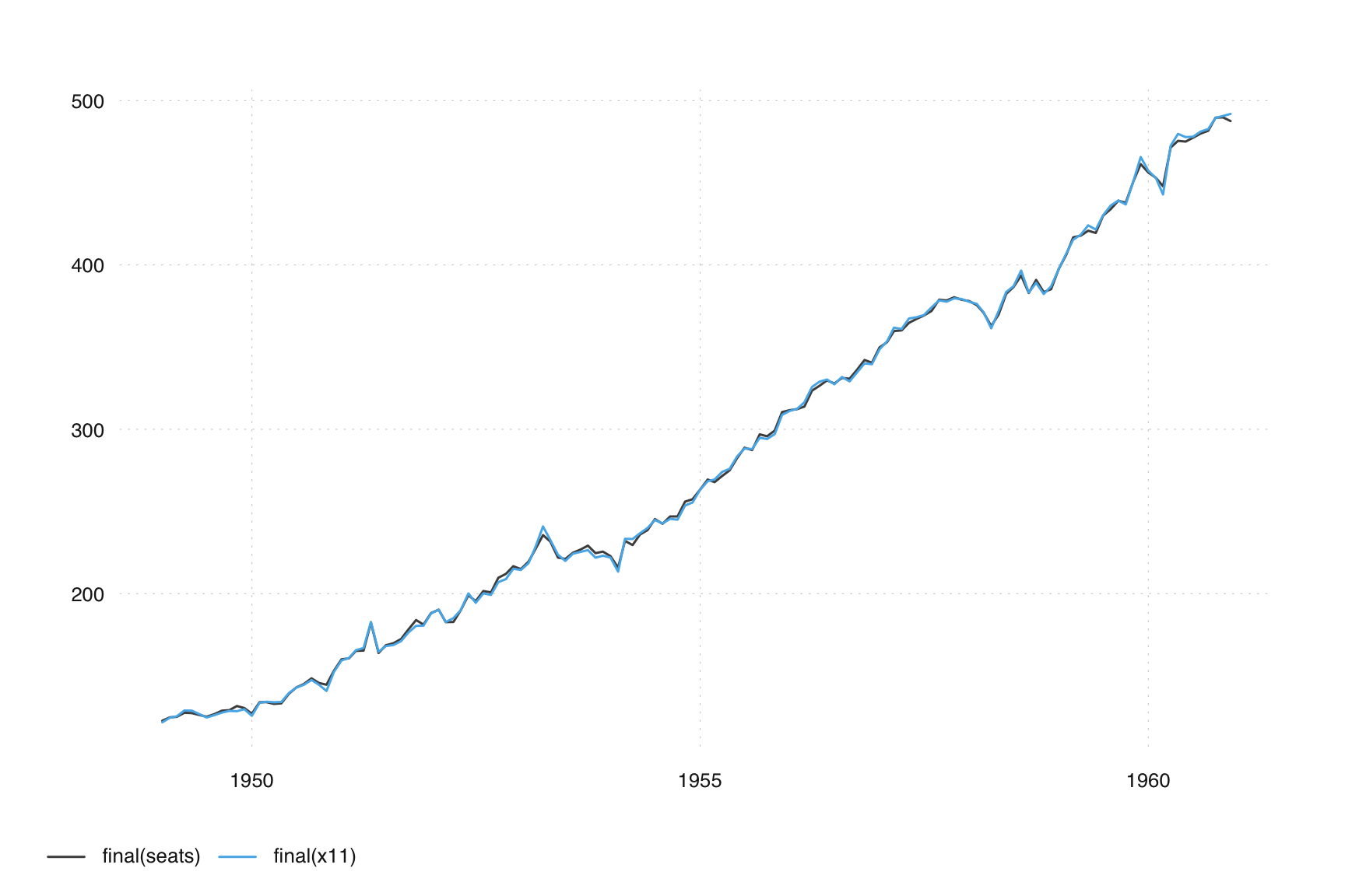
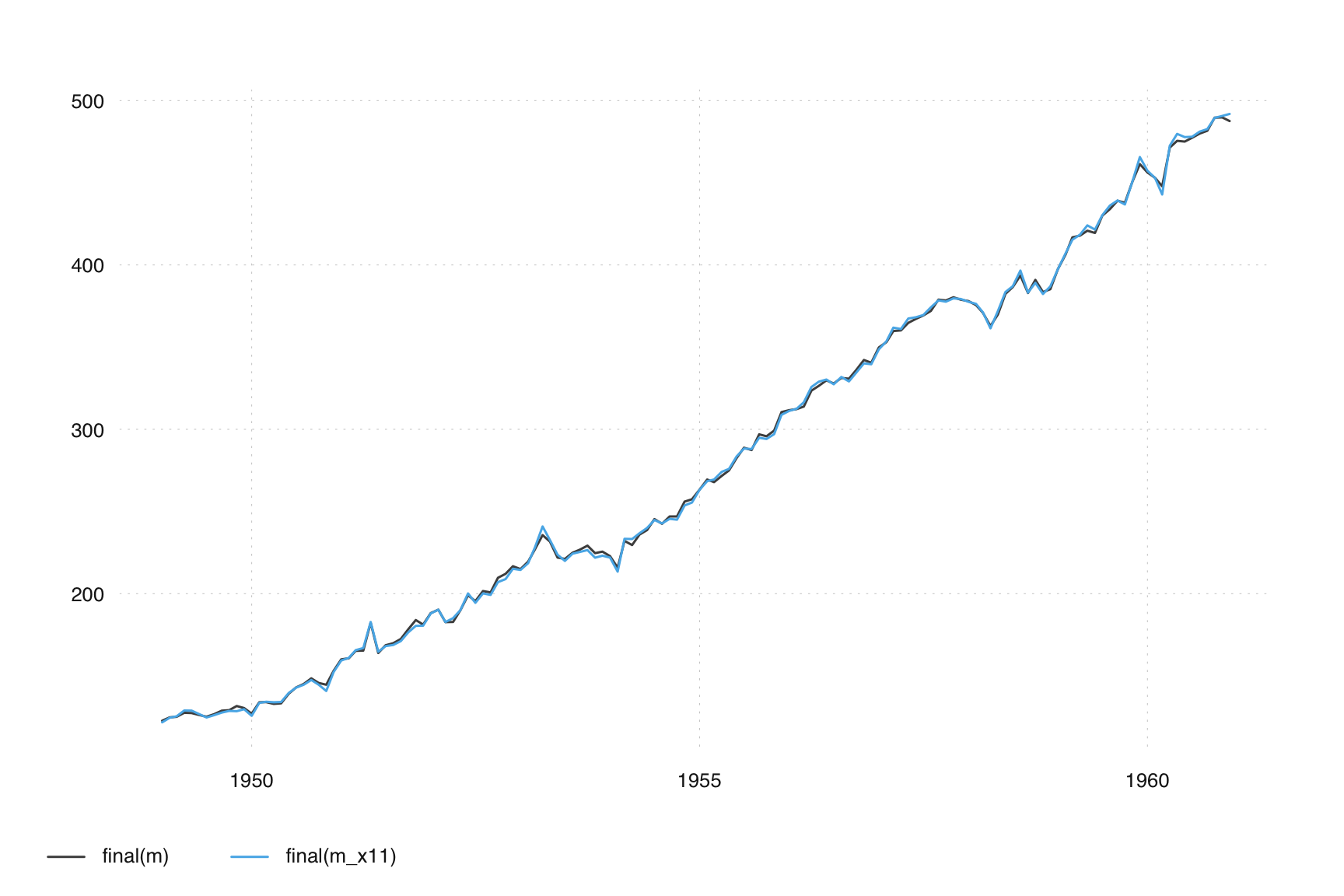
As long as SEATS and X-11 use similar filters, the final adjustment will be similar. Using the default arguments of seas() on AirPassengers, the adjustment is very similar:
We will look into the similarities between SEATS and X-11 in section …
7.2 ARIMA Model decompostion
Given a certain ARIMA model (such as the “Airline” (0 1 1)(0 1 1) which is appropriate for the description of the AirPassengers time series), SEATS decomposes the model into separate models for the trend, the seasonal and the irregular component. This is done by the Canonical Decomposition and will be discussed in Section 7.4.3.
For a given set of ARIMA model parameter, the decomposition of the ARIMA model is almost independent of the data. For each ARIMA specification, there is a unique canonical decomposition. For an “Airline” (0 1 1)(0 1 1) model (with both moving average coefficients not being to close to 1), the trend component can be described with a (0 2 2)(0 0 0) model, while the seasonal sum of seasonal component can be described by a (0 0 11)(0 0 0) model. The parameters of these models can be derived from the parameter estimates of the initial airline model that describes the original series. The irregular component is usually white noise, described by the trivial (0 0 0)(0 0 0) model.
The decomposed ARIMA models imply a certain filter, which is derived by the Wiener-Kolmogorov procedure (Section 7.4.4).
7.3 Comparing SEATS with X-11 filters
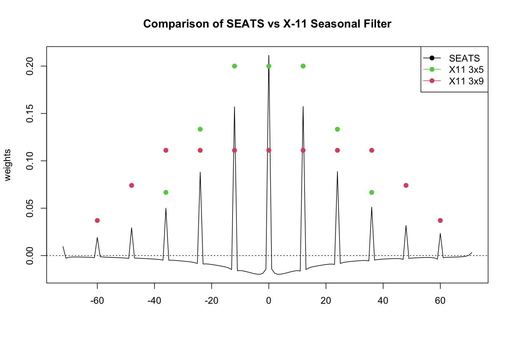
Planas and Depoutot (2002) systematically compare SEATS and X-11 filters and show which X11 seasonal filter that is closest to an implied (0 1 1)(0 1 1) “Airline” SEATS model based on the \(\Theta\). As a reminder, \(\Theta\) refers to the seasonal moving average parameter of the ARIMA model.
Planas, Christophe, and Raoul Depoutot. 2002. “Controlling Revisions in Arima-Model-Based Seasonal Adjustment.”Journal of Time Series Analysis 23 (2): 193–213.
Filter
Closest Seasonal MA
Seasonal MA Interval
3x3
0.364 - 0.400
0.0 - 0.5
3x5
0.543 - 0.563
0.51 - 0.74
3x9
0.723 - 0.732
0.75 - 0.87
3x15
0.824 - 0.828
0.88 - 1.00
Let’s consider small vs large values of seasonal \(\Theta\). Values of \(\Theta\) close to zero yield a seasonal adjustment filter that has seasonal factors that change rapidly over time. This provides considerable smoothing and large revisions. These revisions will only last for a small number of years due to the shorter filters.
Values of \(\Theta\) close to one yield a seasonal adjustment filter that has seasonal factors that change slowly over time. This provides less smoothing but relatively small revisions. Any revisions that do occur will last for a longer period of time due to the longer filters.
Overall, we may think of SEATS filters as a broader, more flexible set of filters than X-11 filers. While we have just seven filters in X-11, we have an infinite number of filters in SEATS. They cover a larger range of filters spans, ranging from filters that are much narrower than X-11 to filters that are much wider.
SEATS greatest strength is also its greatest weakness. As we will see in the example below, SEATS sometimes chooses a filter that is very narrow. From a SEATS perspective, this makes sense: Given an ARIMA model with a very weak seasonality, the filter lengths should be chooses narrowly. From a practical perspective, the resulting seasonal component is undesirable. It is too volatile, essentially catching much of the irregular component and making the resulting seasonally adjusted series too smooth.
7.4 Advanced theory
7.4.1 Quick refresher on ARIMA models and notation
The remaining of the SEATS section will heavily rely on the auto-regressive and moving-average operators \(\phi(B)\) and \(\theta(B)\) where \(B X_t = X_{t-1}\).
If \(X_t\) follows and ARIMA(\(p\), \(d\), \(q\)) model: \[
\phi(B) X_t = \theta(B) a_t
\]
and all model information is contained in \(\phi(B)\) and \(\theta(B)\). Moreover, for any specified \(\phi(B)\) and \(\theta(B)\) that satisfy certain causality criteria there exists a unique Wold decomposition \[
\phi(B) X_t = \theta(B) a_t
\]
The linearized series can be represented by an ARIMA model which captures the stochastic structure of the series. As a reminder, the linearized series is the series with regression effects removed.
After differencing each with the ARIMA’s differencing polynomial, the components are orthogonal (uncorrelated)
SEATS decomposes the auto-regressive polynomial by its roots associating them with different latent components. For example, roots near seasonal frequencies are associated with the seasonal component and roots near zero are associated with the trend component. \[
\phi(B) = \phi_T(B) \cdot \phi_S(B) \cdot \phi_R(B).
\]
If the spectra of all components in non-negative the decomposition is admissible, SEATS finds admissible models for components \[ \phi_T(B) T_t = \theta_T(B) a_{T, t} \]\[ \phi_S(B) S_t = \theta_S(B) a_{S, t} \]\[\phi_R(B) R_t = \theta_R(B) a_{R, t} \]
7.4.3 Canonical Decomposition
However, there infinite number of models that yield the same aggregate. The choices differ in how white noise is allocated among the components. This is where the Canonical Decomposition comes into play. SEATS uses the method of Pierce, Box-Hillmer, Tiao and Burman:
Put all the white noise into the irregular components
Maximize the variance of the irregular
Minimizes the variance of the stationary transforms of the other components
This is called the Canonical Decomposition. We already stated that both X-11 and SEATS estimate the unobserved components by passing a moving-average filter over the observed data. So how do we use these implied component models to get a linear filter? It should be clear that the filter weights will depend on that arima model is picked \(X_t = \Psi(B) a_t\), and what the implied seasonal model, \(\phi_S(B) S_t = \theta_S(B) a_{S,t} \Rightarrow S_t = \Psi(B) a_t\), is.
7.4.4 Wiener-Kolmogorov Algorithm
The Wiener-Kolmogorov (WK) algorithm outlines the methodology to get the so-called WK filter. This is the filter that is equal to the conditional expectation of the seasonal component conditional on the observed series.
\[\widehat{S}_t = \underbrace{\left[ \frac{\Sigma_S}{\Sigma} \frac{\Psi_S(B)\Psi_S(F)}{\Psi(B)\Psi(F)} \right]}_{\mbox{WK filter weights}} X_t\] where \(F=B^{-1}\) if the forward shift operator such that \(F X_t = X_{t+1}\).
More than other coefficients, the seasonal MA (\(\theta_{12}\)) influences whether estimated seasonal factors change either slowly over time (\(\theta_{12}\) close to 1) or rapidly over time (\(\theta_{12}\) close to zero).
7.4.5 Transitory component
Sometimes SEATS includes a transitory component in its decomposition:
\[ X_t = T_t + S_t + R_t + I_t \]
The transitory component captures short, erratic behavior that is not white noise, sometimes associated with awkward frequencies.
The variation from the transitory component should not contaminate the trend or seasonal, and removing it allows SEATS to obtain smoother, more stable trends and seasonal components.
In the final decomposition, the transitory and irregular components are usually combined.
SEATS does not always estimate a transitory component
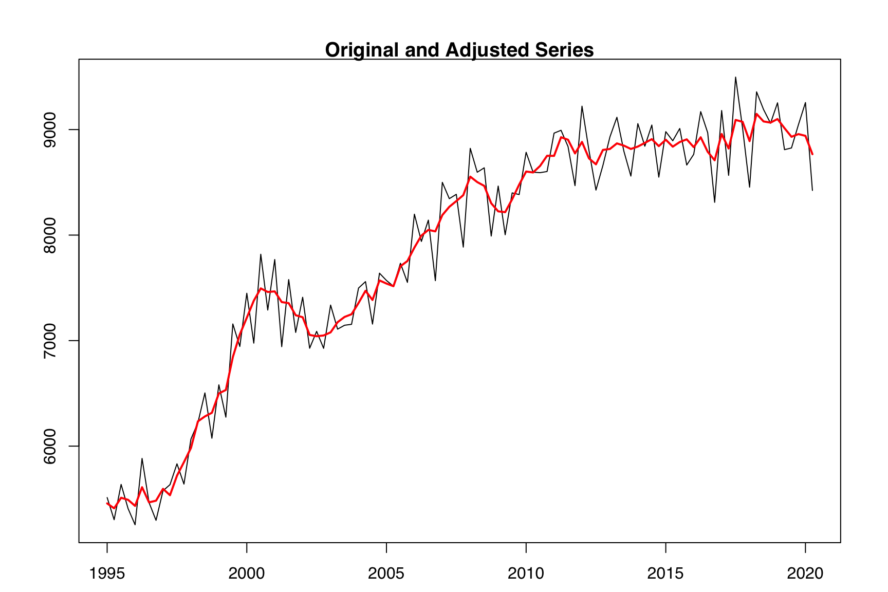
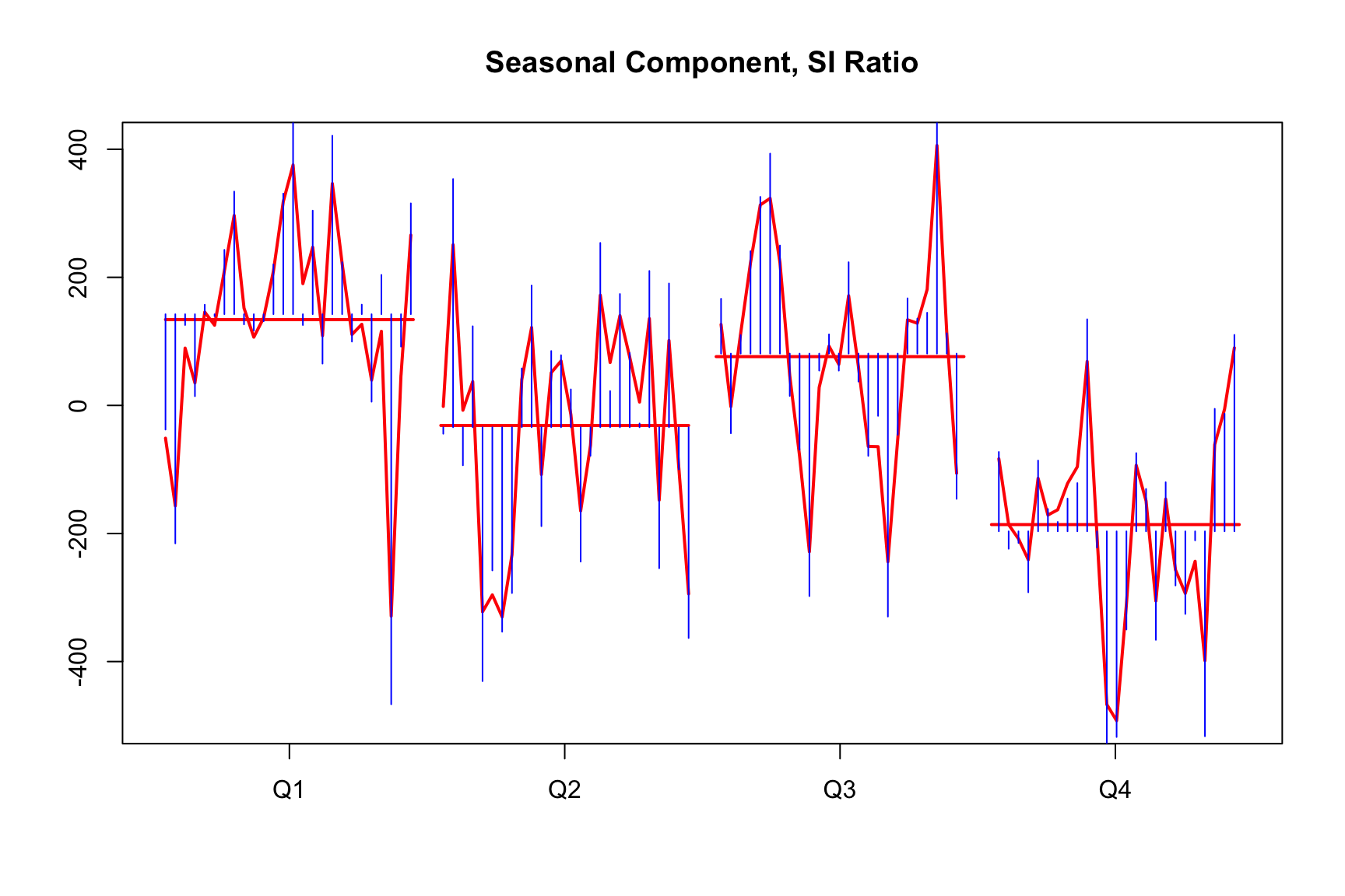
7.5 Case study: narrow SEATS filters
Case Study
Let’s have a look at nominal taxes from Swiss production account.
To me (Christoph), this seems against the very basic idea of seasonal adjustment: We want to collect predictable fluctuations in the seasonal component, not random noise. The other side of the coin is a very smooth seasonal adjustment.
These kind of SI-ratios appear in around 10 to 20% of SEATS adjustment and may be the reason why SEATS often seems smoother than X11.
How to detect these cases? How to deal with these adjustments?
7.6 Considerations when using SEATS in X-13
Some model limitations when using SEATS are as follows.
SEATS does not accept missing lag models. Hence, it is acceptable to specify a (0 1 3)(0 1 1) model but unacceptable to specify (0 1 [1 3])(0 1 1).
The AR and MA orders (p and q) cannot be greater than 3.
Inadmissible decomposition: Sometimes, the estimated values of coefficients make it impossible to estimate components from the estimated ARIMA models. SEATS will usually change the model and re-estimate it in order to get an admissible decomposition. When it is difficult to find an admissible decomposition the airline model is often used as a replacement. This usually gives acceptable results for a broad range of series.
Model span can have large implications in a SEATS adjustment. This is due to the changing dynamics of long time series and how SEATS derives its filters.
7.7 Comparing X-11 and SEATS
The Bureau of Labor Statistics formed a group to do a comparison study between X-11 and model-based seasonal adjustments (CITE BLS 2007). The examined a cross section of 87 BLS series with X-11, SEATS, and STAMP using spectral, revisions history, model adequacy and sliding spans diagnostics. They found that SEATS seasonal factors are usually more stable than X-11 and X-11 trend component is usually more stable than SEATS. Also, among series that were seasonal, residual seasonality almost never appears using either method.
The only exception being a small number of SEATS runs where model inadequacy for the full span of data was present. This manifested as SEATS having difficulty identifying a usable model for decomposition and falling back on the airline model. They found even in these situations the SEATS seasonal adjustment is usually reasonable.
Overall, X-11 and SEATS seasonal adjustments are very similar for many series. SEATS adjustments are often smoother than X-11 seasonal adjustments. For some series, the variance can be different based on the month or season. For example, U.S. Housing Starts is more variable in the winter months than in the summer due to the differences in warm and cold winters. ARIMA model-based seasonal adjustment does not handle this situation very well and assumes a constant variance and the SEATS adjustment wont compensate for this.
7.7.1 SEATS filters from seas output
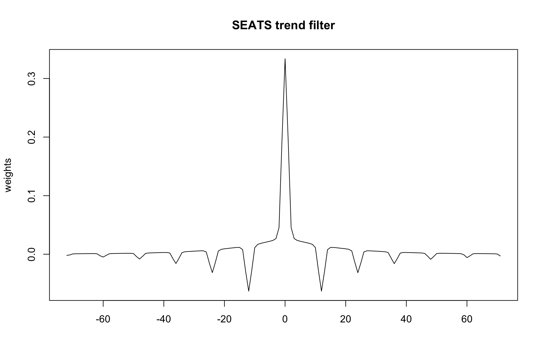
The trend filter and seasonal adjustment filter can be extracted from the output of a seasonal run. This is done via the save argument in the seats spec. In the following example the symmetric trend filter is saved and then exported. Note the finite='yes' argument must be specified to save filter weights.
m<-seas(AirPassengers, seats.finite ='yes', seats.save ='ftf', # symmetric finite trend filter out =TRUE)ftf_file<-file.path(m$wdir, 'iofile.ftf')# reads in filter weights from ftf_filew<-read.delim(textConnection(readLines(ftf_file)[-2]), header =TRUE, stringsAsFactors =FALSE)plot(-72:71, w[,2], type ="l", xlab ="", ylab ="weights", main ="SEATS trend filter")
The default SEATS output tables do not allow users to save the seasonal filter, only the seasonal adjustment and trend filters. Some additional work can be done to calculate the seasonal filters via the canonical decomposition implied models and the Wiener-Kolmogorov algorithm. The code provided here is a bit complicated and will be improved/modularized in subsequent version of this textbook. It involves outputting the mdc table and the using the grep functions to extract salient features for each model component. The naming conventions for the mdc table follow the Wald decomposition notation where moving average components appear in the numerator and differencing and/or autoregressive components appear in the denominator. The following assumes there are no AR components and anything appearing in the denominator is attributed to the differencing operator.
To further understand these components the implied trend model is the following:
macoefs#> [1] 0.04751813 -0.95248187
which tells us the trend is an MA(2) with coefficients \(\theta_1 = 0.04751813\) and \(\theta_2 = -0.95248187\). The variance of the innovations, \(\sigma\) is
trend.var#> [1] 0.05400767
and the differencing is
trendDiff#> [1] 1 -2 1
which is second differencing, i.e. \(\delta(B) = 1 - 2B + B^2 = (1-B)^2\).
We can use these component models to apply the WK algorithm and get the seasonal filter weights. The details of this complex operation are omitted here but a plot of the seasonal filter weights is given in Figure ???.
7.7.2 Reasons for using SEATS or X11
TODO
Add Table with pros and cons
First off, there does not exist a simple flow chat that tells each individual users whether they should use SEATS or X-11. For most well-behaved series both methods will produce suitable seasonal adjustments that will work for the majority of use cases. The ultimate decision between the two comes down to a few questions.
What will you be doing with these seasonal adjustments?
How often is your data revised?
Does your agency have a policy to freeze data/seasonal adjustment revisions after a fixed period of time?
How much time can be devoted to development of initial spec files?
How much time can be devoted to maintenance of spec files?
What is your maintenance schedule? (yearly, monthly, etc)
What are the consequences of a poor adjustment?
What are the consequences of large revisions?
Will your agency be publishing original series, just SA, trends, seasonal factors?
Is there an emphasis on deep methodological understanding of the procedures?
Is there an emphasis on training users of released data to have a methodological understanding of the SA process?
When applied properly (good ARIMA model, filters are not too narrow), it produces a seasonal component that is more stable. This leads to less revisions in the resulting series.
When applied improperly (bad ARIMA model, narrow filters), it produces an unpredictable seasonal component and an overly smooth seasonally adjusted series.
X-11 is more ‘robust’: If applied without additional checks. If this is desirable it may be a better option.
If you check SEATS models carefully, it may produce a more stable adjustment.
To sum up, whether you should use SEATS or X11 also depends on how much work you are willing to invest in a series.