flowchart TD
  A[RegARIMA Modeling] --> B(Model Comparison / Diagnostics)
  B --> A
  A --> C[Seasonal Adjustment]
  C --> D[Seasonal Adjustment Diagnostics]
  D --> C
  D --> A
5 regARIMA Model
An ARIMA model with external regressors (regARIMA) lies at the heart of many of the procedures in X-13. As we have seen in Chapter 3, regARIMA consists of several interacting specs. Some of the these specs will be further detailed in Chapter 8, Chapter 9, and Chapter 10 (Holidays, Trading Days, and Outliers).
Like most statistical modeling in X-13, the process of finding the best model is iterative. Analysts use statistical tools and their expertise to fine-tune the regARIMA model. This iterative process is visualized in the flow chart below.
Once a satisfying regARIMA has been found, one proceeds to the seasonal adjustment step. The regARIMA model is crucial in forecasting the time series for applying symmetric filters and extracting components, whether using SEATS or X-11 for seasonal adjustment. In addition, in SEATS, the ARIMA model is also used to derive trend, seasonal, and irregular components.
The regARIMA model also includes exogenous information or regressors, like holiday effects, additive outliers, and level shifts. These elements help in forecasting and analyzing the series. For example, regARIMA modeling can answer if a series is affected by trading day effects or how outliers impact results. It’s also used to integrate external regression variables such as moving holidays and trading day effects into the analysis.
5.1 ARIMA Basics
The regARIMA model combines two elements: regression and ARIMA. The ARIMA segment itself is composed of a differencing order (the “I”, for “integrated”) and the ARMA part. This chapter aims to simplify these concepts without getting too technical, providing enough understanding for effective seasonal adjustment.
ARIMA stands for Autoregressive Integrated Moving Average. “Autoregressive” (AR) means the model uses past values of the series to predict the current value. For instance, an AR(1) model uses one lagged value:
\[ Y_t = \phi Y_{t-1} + a_t \]
Here, \(Y_t\) is the time series, \(\phi\) a coefficient, and \(\{a_t\}\) an uncorrelated sequence of errors.1
An AR(p) model extends this to \(p\) lagged values:
\[ Y_t = \phi_1 Y_{t-1} + \phi_2 Y_{t-2} + \cdots + \phi_p Y_{t-p} + a_t \]
where now we have \(p\) coefficients \(\phi_1, \phi_2, \ldots, \phi_p\) to be estimated.
The “Moving Average” (MA) part uses past errors of the series for prediction. An MA(1) model looks like:
\[ Y_t = a_t + \theta a_{t-1} \]
and uses the current and one lagged error term.2
An MA(q) model includes \(q\) lagged error terms:
\[ Y_t = a_t + \theta_1 a_{t-1} + \theta_2 a_{t-2} + \cdots + \theta_q a_{t-q} \].
An ARMA(p, q) model combines these AR and MA components, using \(p\) lagged values of the series and \(q\) lagged error terms. In practice, X13’s automatic modeling usually finds appropriate \(p\) and \(q\) values. However, it is worth paying attention to correctly set the differencing and regression variables for seasonal adjustment.
5.2 Differencing
ARMA models are most effective with stationary time series, where both the mean and correlation structure do not vary over time. For non-stationary time series, transforming them into stationary ones is essential, and differencing is a widely used method for this purpose. It is known that differencing a series \(k\) times can remove a polynomial trend of degree \(k\). Therefore, the first differencing is effective for a series with a linear trend, while the second differencing works for a series with a quadratic trend.
Seasonal patterns might also require seasonal differencing to achieve stationarity. The orders of differencing for the non-seasonal and seasonal parts are denoted as \(d\) and \(D\), respectively. Combining these with the stochastic model specification gives the notation SARIMA(p, d, q)(P, D, Q), where \(p\), \(d\), \(q\) are non-seasonal parameters, and \(P\), \(D\), \(Q\) are seasonal.3:
3 The “S” in SARIMA stands for seasonal. Since most of the ARIMA models within X-13 are seasonal, we will restrain from using the term and usually refer to an ARIMA model of the structure (p, d, q)(P, D, Q).
\[\text{SARIMA}\underbrace{(p, d, q)}_{\text{non-seasonal }}\underbrace{(P, D, Q)}_{\text{seasonal}}.\]
Let’s apply this to AirPassengers. A log-transformed version of the series looks as follows:
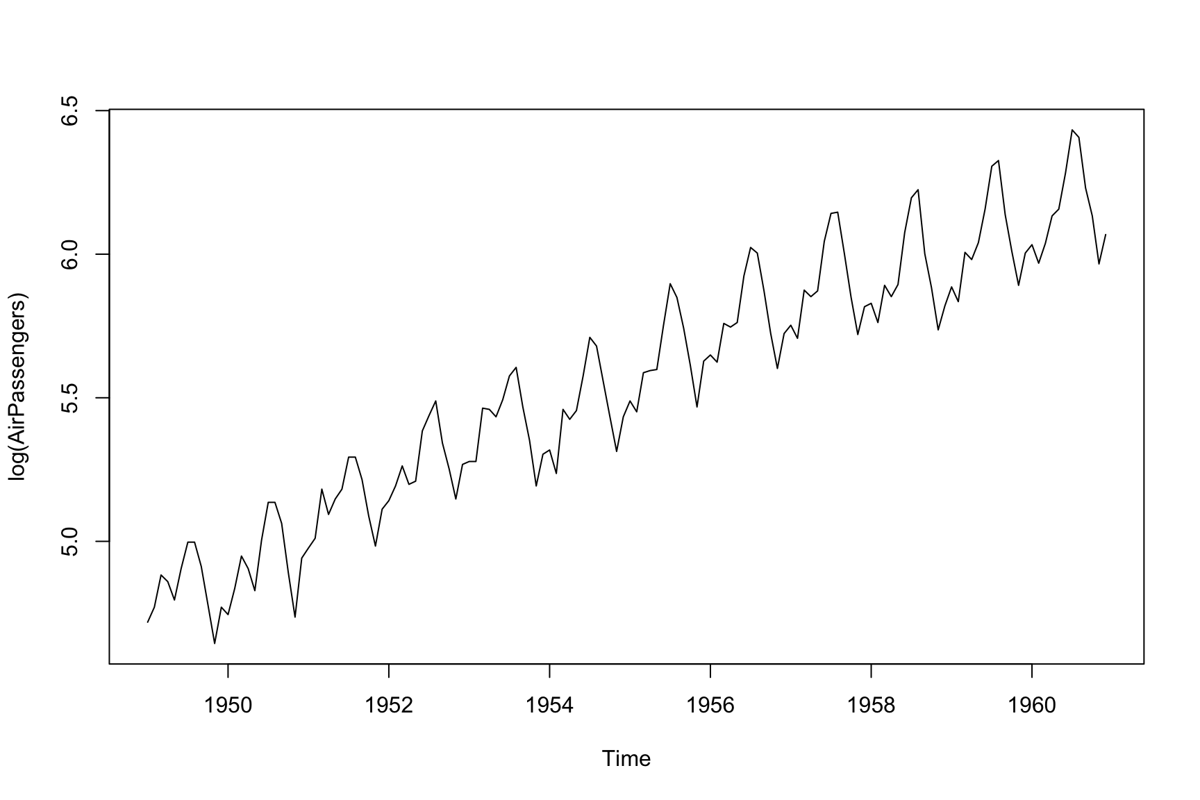
This series exhibits a clear increasing trend and seasonal pattern. Let’s call the log-transformed series \(X_t\). We can now difference the series to make \(Y_t = \Delta X_t = X_t - X_{t-1}\). Which looks like:
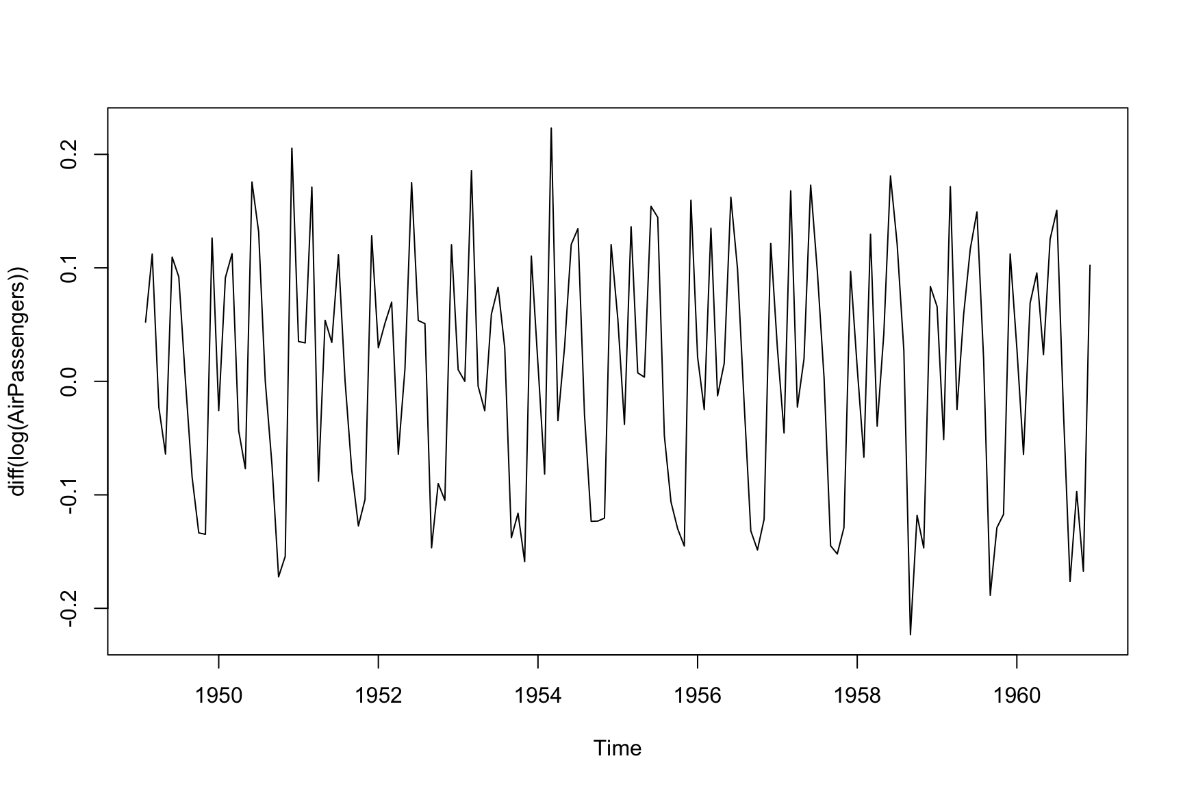
The trend is removed, but some seasonal patterns remain. Seasonal differencing is then applied to the already first differenced series \(Y_t\):
\[ Z_t = Y_t - Y_{t-12} \]
A plot of \(Z_t\):
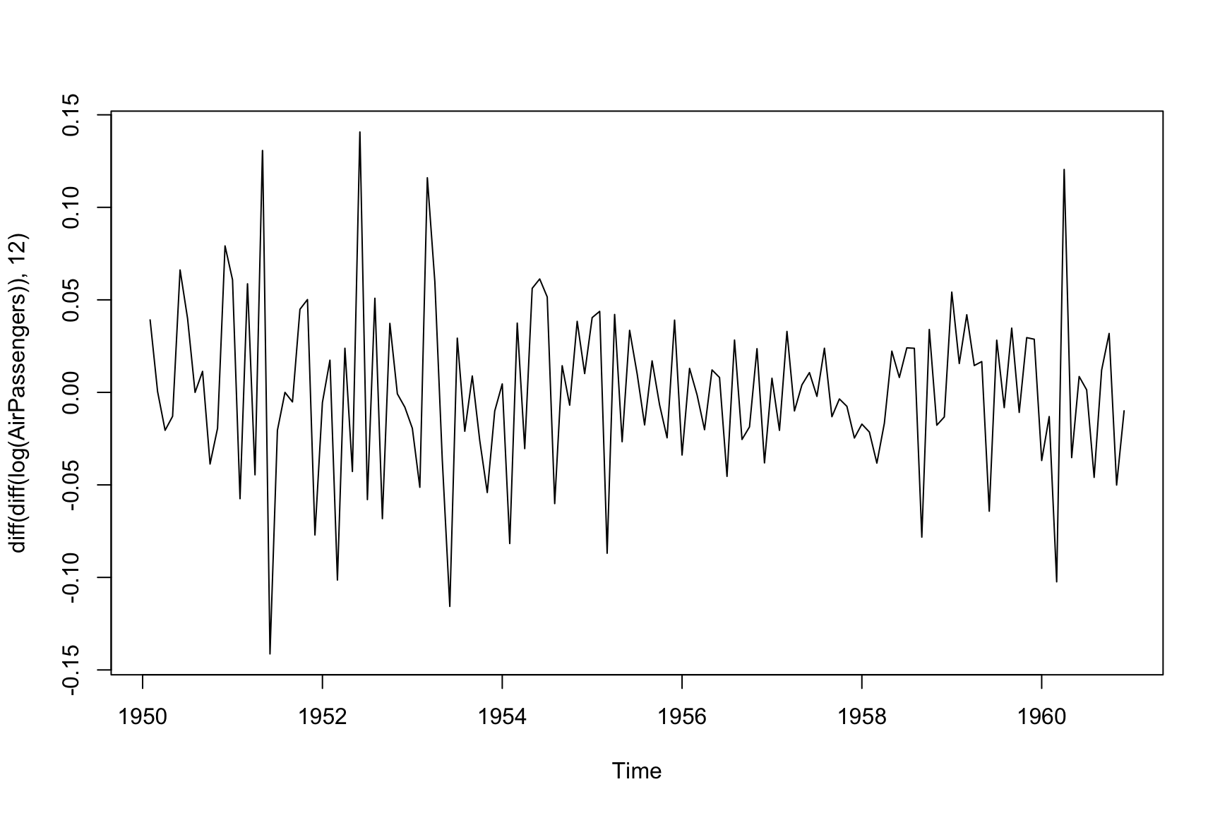
Now, both the linear trend and seasonal patterns are removed, leaving a stationary process suitable for modeling with an (0, 0, 1)(0, 0, 1) ARIMA model. When the differencing order for both seasonal and non-seasonal components is included, the model becomes (0, 1, 1)(0, 1, 1), often called the “airline model” after Box and Jenkins’ work.4
4 The “airline model,” or the ARIMA(0, 1, 1)(0, 1, 1) model, was popularized by Box and Jenkins (1970) through their influential work in the field of time series analysis. This model is often associated with their seminal book “Time Series Analysis: Forecasting and Control.” First published in 1970, this book has been a foundational text in the field of time series analysis. The airline model, named for its application in modeling airline passenger data, exemplifies the application of Seasonal ARIMA modeling in practical scenarios.
Box, George E. P., and Gwilym M. Jenkins. 1970. Time Series Analysis: Forecasting and Control. San Francisco: Holden-Day.
5.3 Automated ARIMA modeling
By default, seas() invokes the automdl spec to perform an automated ARIMA model search.
Unsurprisingly, the basic call to seas(AirPassengers) opts for the (0, 1, 1)(0, 1, 1) “airline model” that has its name from the series:
m <- seas(AirPassengers)
summary(m)
#>
#> Call:
#> seas(x = AirPassengers)
#>
#> Coefficients:
#>                     Estimate Std. Error z value Pr(>|z|)
#> Weekday           -0.0029497  0.0005232  -5.638 1.72e-08 ***
#> Easter[1]          0.0177674  0.0071580   2.482   0.0131 *
#> AO1951.May         0.1001558  0.0204387   4.900 9.57e-07 ***
#> MA-Nonseasonal-01  0.1156204  0.0858588   1.347   0.1781
#> MA-Seasonal-12     0.4973600  0.0774677   6.420 1.36e-10 ***
#> ---
#> Signif. codes:  0 '***' 0.001 '**' 0.01 '*' 0.05 '.' 0.1 ' ' 1
#>
#> SEATS adj.  ARIMA: (0 1 1)(0 1 1)  Obs.: 144  Transform: log
#> AICc: 947.3, BIC: 963.9  QS (no seasonality in final):    0
#> Box-Ljung (no autocorr.): 26.65   Shapiro (normality): 0.9908
Technically, model identification starts with determining the appropriate level of differencing, both seasonal and non-seasonal. Following this, the procedure compares various ARIMA models and opts for one with a low information criterion. The fivebestmdl() function can be used to look into some contenders for ‘good models’. These models are ranked based on their Bayesian Information Criterion (BIC):
fivebestmdl(m)
#>            arima    bic
#> 1 (0 1 0)(0 1 1) -4.007
#> 2 (1 1 1)(0 1 1) -3.986
#> 3 (0 1 1)(0 1 1) -3.979
#> 4 (1 1 0)(0 1 1) -3.977
#> 5 (0 1 2)(0 1 1) -3.970
5.4 Regression
After ARIMA and differencing, the final element of regARIMA is the regression component. The regression component describes the effect of exogenous variables on the residuals of an ARIMA model.
If no transformation or intervention is needed, the regARIMA model takes the following form:5
The left-hand side of an regARIMA can be transformed and adjusted for subjective interventions. In such cases, the regARIMA formula extends to:
\[ f\left(\frac{Y_t}{D_t} \right) = \boldsymbol{\beta}^\prime {\mathbf X}_t + Z_t \]
The function \(f\) represents a transformation, with the logarithmic transformation (\(f(x) = \log(x)\)) being a common choice. \(D_t\) represents any interventions applied before transformation or modeling. These interventions are often specific to each time series and are applied based on the unique circumstances of the data. For example, if an event like a soybean farmer strike affects the data series, this intervention can help adjust the data before further analysis.
\[ Y_t = \underbrace{\boldsymbol{\beta}^\prime {\mathbf X}_t}_{\text{regression}} + \underbrace{Z_t}_{\text{ARIMA}} \]
In this model, \(Y_t\) is the observed time series. The regression component is \({\mathbf X}_t\) and \(Z_t\) represents the ARIMA process. The key difference between a regARIMA model and classical linear models is the assumption about \(Z_t\). In regARIMA, \(Z_t\) is an ARIMA process, where in classic models the error terms are typically assumed to be uncorrelated.
For effective seasonal adjustment, it’s crucial to accurately specify the regARIMA model. Often, the automated modeling capabilities of X-13 are sufficient for determining a suitable model. This auto-generated model can also act as a starting point for further refinement of the regARIMA model. The seasonal package incorporates the automatic identification feature by default, and makes the process user-friendly and streamlined.
5.5 Automated regressor identification
By default, the seas() command performs various automated regressor tests:
- Outlier
- Irregular Holidays (Easter)
- Weekday regressors
For example, the basic call to seas() reveals the presence of Weekday, Easter and Outlier effects in the AirPassengers data:
summary(seas(AirPassengers))
#>
#> Call:
#> seas(x = AirPassengers)
#>
#> Coefficients:
#>                     Estimate Std. Error z value Pr(>|z|)
#> Weekday           -0.0029497  0.0005232  -5.638 1.72e-08 ***
#> Easter[1]          0.0177674  0.0071580   2.482   0.0131 *
#> AO1951.May         0.1001558  0.0204387   4.900 9.57e-07 ***
#> MA-Nonseasonal-01  0.1156204  0.0858588   1.347   0.1781
#> MA-Seasonal-12     0.4973600  0.0774677   6.420 1.36e-10 ***
#> ---
#> Signif. codes:  0 '***' 0.001 '**' 0.01 '*' 0.05 '.' 0.1 ' ' 1
#>
#> SEATS adj.  ARIMA: (0 1 1)(0 1 1)  Obs.: 144  Transform: log
#> AICc: 947.3, BIC: 963.9  QS (no seasonality in final):    0
#> Box-Ljung (no autocorr.): 26.65   Shapiro (normality): 0.9908
We will cover these regressors in more detail in later chapters. The decision whether to include a regressor is typically left to an augmented AICc test, which we already covered in Section 4.2.
In production, the general rule is to not use automatic modeling. This implies that if you plan to include seasonal adjustment as part of a regular, large-scale data processing routine (such as monthly operations), it’s not recommended to run automatic model identification each month. A better approach is to use automatic model selection once and then set the chosen model permanently in the specification. The static() function from the seasonal package can automate this process.
5.6 Example: AirPassengers
Once again, consider the default seasonal adjustment:
m1 <- seas(AirPassengers, x11 = "")
summary(m1)
#>
#> Call:
#> seas(x = AirPassengers, x11 = "")
#>
#> Coefficients:
#>                     Estimate Std. Error z value Pr(>|z|)
#> Weekday           -0.0029497  0.0005232  -5.638 1.72e-08 ***
#> Easter[1]          0.0177674  0.0071580   2.482   0.0131 *
#> AO1951.May         0.1001558  0.0204387   4.900 9.57e-07 ***
#> MA-Nonseasonal-01  0.1156204  0.0858588   1.347   0.1781
#> MA-Seasonal-12     0.4973600  0.0774677   6.420 1.36e-10 ***
#> ---
#> Signif. codes:  0 '***' 0.001 '**' 0.01 '*' 0.05 '.' 0.1 ' ' 1
#>
#> X11 adj.  ARIMA: (0 1 1)(0 1 1)  Obs.: 144  Transform: log
#> AICc: 947.3, BIC: 963.9  QS (no seasonality in final):    0
#> Box-Ljung (no autocorr.): 26.65   Shapiro (normality): 0.9908
#> Messages generated by X-13:
#> Warnings:
#> - Visually significant seasonal and trading day peaks have
#>   been found in one or more of the estimated spectra.
This time, we are using the X-11 method, rather than SEATS, which is the default in seasonal. (We will cover the distinction between X-11 and SEATS in the next chapters.) We can see from the summary that X-13 has opted for an (0 1 1)(0 1 1) ARIMA model. The udg() is an accessor function for many statistics, and can be used to extract the model directly:
seasonal::udg(m, "automdl")
#>          automdl
#> "(0 1 1)(0 1 1)"
If we want to hard-code this model for subsequent runs, and turn off automatic model identification, this can be done via
static(m1)
#> seas(
#>   x = AirPassengers,
#>   x11 = "",
#>   regression.variables = c("td1coef", "easter[1]", "ao1951.May"),
#>   arima.model = "(0 1 1)(0 1 1)",
#>   regression.aictest = NULL,
#>   outlier = NULL,
#>   transform.function = "log"
#> )
If you run this code in R, you will get the same result as with the original specification.
seasonal allows you to use all options available in X-13. In the following, we want to explore the use of outlier.span to fine-tune automated outlier detection. With the span option, you can limit the outlier detection to a certain time span. Note from previous chapters that we combine spec names and spec arguments by a dot (.).
We also set outlier.critical manually to override the default value that adjusts to the length of the outlier span:
m_span <- seas(
  AirPassengers,
  outlier.critical = 4.0,
  outlier.span = "1958.jan, "
)
summary(m_span)
#>
#> Call:
#> seas(x = AirPassengers, outlier.critical = 4, outlier.span = "1958.jan, ")
#>
#> Coefficients:
#>                    Estimate Std. Error z value Pr(>|z|)
#> Weekday           -0.002644   0.000604  -4.377 1.20e-05 ***
#> Easter[1]          0.021321   0.008395   2.540  0.01110 *
#> MA-Nonseasonal-01  0.235404   0.083756   2.811  0.00495 **
#> MA-Seasonal-12     0.543743   0.074644   7.284 3.23e-13 ***
#> ---
#> Signif. codes:  0 '***' 0.001 '**' 0.01 '*' 0.05 '.' 0.1 ' ' 1
#>
#> SEATS adj.  ARIMA: (0 1 1)(0 1 1)  Obs.: 144  Transform: log
#> AICc: 965.3, BIC: 979.2  QS (no seasonality in final):    0
#> Box-Ljung (no autocorr.): 28.26   Shapiro (normality): 0.9829 .
m_nospan <- seas(
AirPassengers,
outlier.critical = 4.0
)
summary(m_nospan)
#>
#> Call:
#> seas(x = AirPassengers, outlier.critical = 4)
#>
#> Coefficients:
#> Estimate Std. Error z value Pr(>|z|)
#> Weekday -0.0029497 0.0005232 -5.638 1.72e-08 ***
#> Easter[1] 0.0177674 0.0071580 2.482 0.0131 *
#> AO1951.May 0.1001558 0.0204387 4.900 9.57e-07 ***
#> MA-Nonseasonal-01 0.1156204 0.0858588 1.347 0.1781
#> MA-Seasonal-12 0.4973600 0.0774677 6.420 1.36e-10 ***
#> ---
#> Signif. codes: 0 '***' 0.001 '**' 0.01 '*' 0.05 '.' 0.1 ' ' 1
#>
#> SEATS adj. ARIMA: (0 1 1)(0 1 1) Obs.: 144 Transform: log
#> AICc: 947.3, BIC: 963.9 QS (no seasonality in final): 0
#> Box-Ljung (no autocorr.): 26.65 Shapiro (normality): 0.9908By limiting the span for outlier detection to the last 3 years, we don’t allow the procedure to detect the additive outlier in 1951. As we can see, small changes in outlier identification can have a substantial effect on the estimated regARIMA parameters.
5.7 Case Study:
Let’s fit a regARIMA model to a series and decide if you should be adding a regression variable that accounts for the number of weekdays vs weekend days in each month. This is known as a 1-coefficient trading day and will be discussed in further detail in Chapter 9. For the sake of this case study we will just need to know that the regression variable is added via the additon of regression.variables = "td1coef" to our seas() function.
Consider the Total Vehicle Miles Traveled series from the fred database. This is the series with id = TRFVOLUSM227NFWA
plot_fred("TRFVOLUSM227NFWA")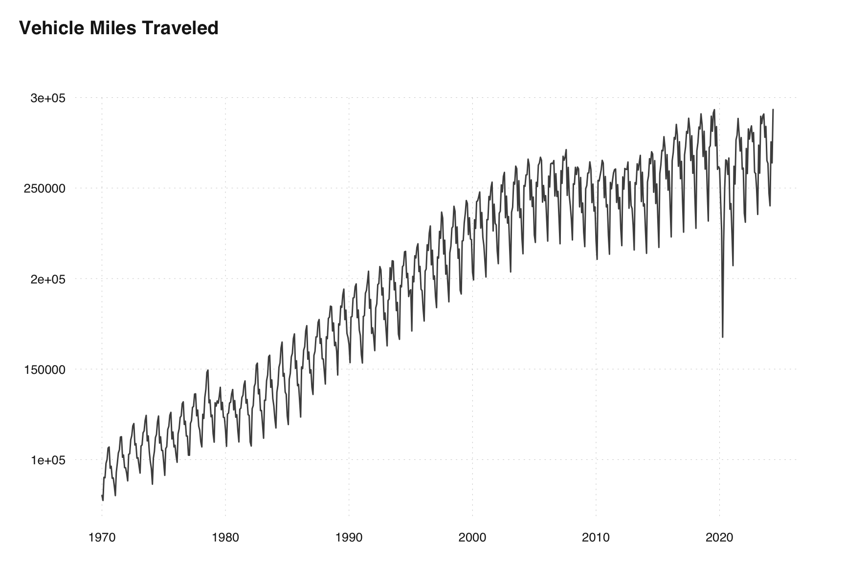
First we can do arima modeling without regressors to see the stocastic structure.
x = ext_fred("TRFVOLUSM227NFWA")
m = seas(x,
         x11 = "",
         outlier = NULL,
         regression.aictest = NULL)
summary(m)
#>
#> Call:
#> seas(x = x, regression.aictest = NULL, outlier = NULL, x11 = "")
#>
#> Coefficients:
#>                   Estimate Std. Error z value Pr(>|z|)
#> AR-Nonseasonal-01  0.36675    0.08144   4.503 6.70e-06 ***
#> MA-Nonseasonal-01  0.53572    0.08070   6.638 3.18e-11 ***
#> MA-Nonseasonal-02  0.27866    0.05264   5.293 1.20e-07 ***
#> MA-Seasonal-12     0.81880    0.02510  32.619  < 2e-16 ***
#> ---
#> Signif. codes:  0 '***' 0.001 '**' 0.01 '*' 0.05 '.' 0.1 ' ' 1
#>
#> X11 adj.  ARIMA: (1 1 2)(0 1 1)  Obs.: 653  Transform: log
#> AICc: 1.261e+04, BIC: 1.264e+04  QS (no seasonality in final):    0
#> Box-Ljung (no autocorr.): 26.53   Shapiro (normality): 0.6782 ***
The automatic modeling identifies an ARIMA(1 1 2)(0 1 1) model. This is a fairly complex non-seasonal model and we will see if this can be simplified without causing any modeling issues. Additionally, it would make sense the number of vehicle miles traveled would be effected by weekday/weekend composition of the month.
m_td = seas(
  x,
  x11 = "",
  outlier = NULL,
  regression.aictest = NULL,
  regression.variables = "td1coef"
)
summary(m_td)
#>
#> Call:
#> seas(x = x, regression.aictest = NULL, outlier = NULL, x11 = "",
#>     regression.variables = "td1coef")
#>
#> Coefficients:
#>                    Estimate Std. Error z value Pr(>|z|)
#> Weekday           0.0008651  0.0002023   4.276 1.90e-05 ***
#> AR-Nonseasonal-01 0.4279865  0.0837257   5.112 3.19e-07 ***
#> MA-Nonseasonal-01 0.6277301  0.0856906   7.326 2.38e-13 ***
#> MA-Nonseasonal-02 0.2059410  0.0567153   3.631 0.000282 ***
#> MA-Seasonal-12    0.8244534  0.0247570  33.302  < 2e-16 ***
#> ---
#> Signif. codes:  0 '***' 0.001 '**' 0.01 '*' 0.05 '.' 0.1 ' ' 1
#>
#> X11 adj.  ARIMA: (1 1 2)(0 1 1)  Obs.: 653  Transform: log
#> AICc: 1.262e+04, BIC: 1.264e+04  QS (no seasonality in final):    0
#> Box-Ljung (no autocorr.): 20.53   Shapiro (normality): 0.678 ***
The trading day regressor is highly significant. We can see this looking at the p-value in the summary table. Now can we get away with a simplier model? Say, the airline model.
m_td_airline = seas(
  x,
  x11 = "",
  outlier = NULL,
  regression.aictest = NULL,
  regression.variables = "td1coef",
  arima.model = "(0 1 1)(0 1 1)"
)
summary(m_td_airline)
#>
#> Call:
#> seas(x = x, regression.aictest = NULL, outlier = NULL, x11 = "",
#>     regression.variables = "td1coef", arima.model = "(0 1 1)(0 1 1)")
#>
#> Coefficients:
#>                    Estimate Std. Error z value Pr(>|z|)
#> Weekday           0.0008731  0.0002126   4.107 4.01e-05 ***
#> MA-Nonseasonal-01 0.1432122  0.0386804   3.702 0.000214 ***
#> MA-Seasonal-12    0.8337828  0.0242370  34.401  < 2e-16 ***
#> ---
#> Signif. codes:  0 '***' 0.001 '**' 0.01 '*' 0.05 '.' 0.1 ' ' 1
#>
#> X11 adj.  ARIMA: (0 1 1)(0 1 1)  Obs.: 653  Transform: log
#> AICc: 1.269e+04, BIC: 1.271e+04  QS (no seasonality in final):    0
#> Box-Ljung (no autocorr.): 74.15 *** Shapiro (normality): 0.6684 ***
Let’s compare AIC values to see which model is preferred.
The AIC of the original model selected is much lower.
5.8 Exercises
-
Performing an automated seasonal adjustment:
- Perform a seasonal adjustment on the
fdeathsdata using the default settings. - Plot the results and summarize the key components of the model.
- Perform a seasonal adjustment on the
-
Inspecting model parameters:
- Inspect the model chosen for the
fdeathsdataset. - Identify the degrees of seasonal and non-seasonal differencing.
- Determine the seasonal and non-seasonal AR and MA orders.
- Inspect the model chosen for the
-
Using the
static()function:- Use the
static()function to extract the static version of the automated model chosen for thefdeathsdataset. - Replace the automatic procedures in the model call with the static choices made by the automated model.
- Use the
-
Bonus: re-estimating using base R: